We show three methods for calculating the coefficients in the multinomial logistic model, namely: (1) using the coefficients described by the r binary models, (2) using Solver and (3) using Newton’s method. On this webpage, we review the first of these methods. See Finding Multinomial Logistic Regression Coefficients using Solver and Finding Multinomial Logistic Regression Coefficients using Newton’s Method.
Example 1: A new drug was tested for the treatment of certain types of cancer patients. Figure 1 shows the data for a sample of 860 patients, 449 male (Gender = 0) and 411 women (Gender = 1) given the cancer treatment at various dosages. Three outcomes were measured after 5 years: the patient was cured (i.e. cancer-free after 5 years), the patient died or the patient was alive but still had cancer.
Build a multinomial logistic regression model based on this data and use it to predict the probability of the three outcomes for men and women at a dosages of 24 mg and 24.5 mg.

Figure 1 – Data for Multinomial Logistic Regression
We use Dead as the reference outcome. Generally, it is best to use the outcome with the largest sample size (400 for Dead), although the end result will be the same if another choice is made. The key components of the model are shown in Figure 2.
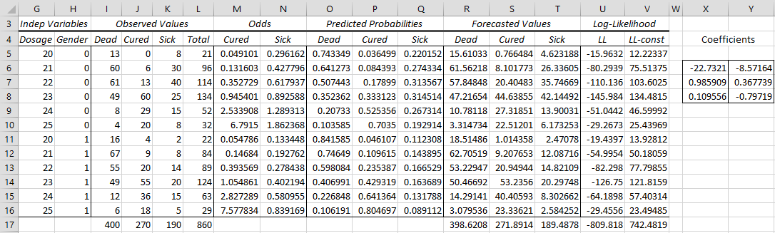
Figure 2 – Multinomial logistic regression model (part 1)
The coefficients are derived from the two binary models: Cured + Dead and Sick + Dead, i.e. the binary logistic regression model based on the data in A5:D16 and the binary logistic regression model based on the data in the range A5:C5 + E5:E16. The fact that the data range for the second model is not contiguous is not a problem since we will be using the Real Statistics MLogitExtract function to extract the correct outcomes from the original data range.
Real Statistics Function: The Real Statistics Resource Pack provides the following array function where R1 is a summary data range for multinomial logistic regression with outcomes for the dependent variable of 0, …, r.
MLogitExtract(R1, r, s, head): fill the highlighted range with the columns defined by string s from the data from R1. The string s takes the form of a comma-delimited list of numbers 0, …, r. If head = TRUE (default) then R1 includes column headings, while if head = FALSE then R1 does not include column headings. Also, the output will contain column headings if head = TRUE and it will contain only data if head = FALSE.
For the Cured + Dead binary model we use the data range MLogitExtract(A4:E16,2,”1,0”) or MLogitExtract(A5:E16,2,”1,0”,False). The first formula includes column headings and the second does not. Here “1,0” means that the data for outcome 1 (column J) is used followed by the data for outcome 0 (column I). The second argument has value 2 since the outcomes are 0, 1, 2. It is important that the reference outcome (i.e. 0) is listed second so that “success” in the binary logistic regression model is for the non-reference outcome.
For the Sick + Dead binary model we use the data range MLogitExtract(A4:E16,2,”2,0”) or MLogitExtract(A5:E16,2,”2,0”,False). The first formula includes column headings and the second does not. The output for MLogitExtract(A4:E16,2,”2,0”) is shown in Figure 3.

Figure 3 – Use of MLogitExtract function
In fact for our purposes here we don’t need to explicitly display the results of the MLogitExtract function. Instead, we use the MLogitExtract formula as an argument in the LogitCoeff Real Statistics formula (see Real Statistics Functions for Multinomial Logistic Regression), which calculates the coefficients for binary logistic regression. In particular, we insert the following array formula in range X6:X8 of Figure 1 to calculate the binary logistic regression coefficients for the Cured + Dead model.
=LogitCoeff(MLogitExtract(A5:E16,2,”1,0″,FALSE))
Similarly, we insert the following array formula in range Y6:Y9 of Figure 1 to calculate the binary logistic regression coefficients for the Sick + Dead model.
=LogitCoeff(MLogitExtract(A5:E16,2,”2,0″,FALSE))
The remaining formulas in Figure 1 are calculated as described in Basic Concepts of Multinomial Logistic Regression. E.g. the formulas used for the cells in row 5 are as shown in Figure 4.
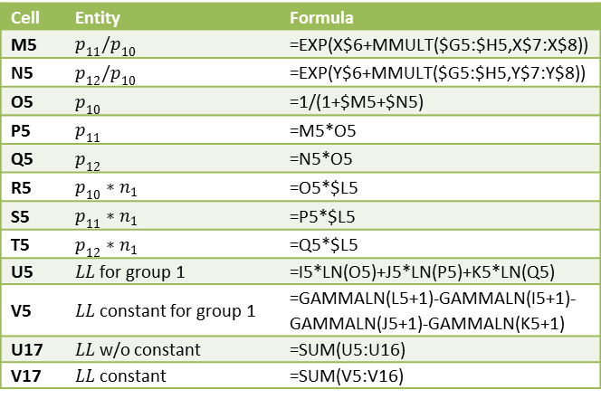 Figure 4 – Key formulas from Figure 1
In calculating cell V5 we use the fact that n! = Γ(n+1) where Γ is the gamma function (per Property 1c of Gamma Function). Thus ln n! = GAMMALN(n+1).
The values of L0, the various pseudo-R2 statistics as well as the chi-square test for the significance of the multinomial logistic regression model are displayed in Figure 5.
")
Figure 5 – Multinomial logistic regression model (part 2)
The significance of the two sets of coefficients are displayed in Figure 6.
")
Figure 5 – Multinomial logistic regression model (part 3)
Here the ranges H22:N24 and H29:N31 can be calculated by the Real Statistics array formulas
=LogitCoeff(MLogitExtract(A5:E16,2,”1,0″,FALSE))
=LogitCoeff(MLogitExtract(A5:E16,2,”2,0″,FALSE))
The forecasted probabilities, based on the above multinomial logistic regression model, of the three outcomes for men and women at dosages of 24 mg and 24.5 mg is displayed in Figure 6.
That exp(bgender) = 1.116 for Cured + Dead means that for any given dosage women are 11.6% more likely than men to be cured rather than dead. That exp(bgender) = .451 for Sick + Dead means that for any given dosage men are 2.22 (= 1/.451) more likely than women to be sick rather than dead. Since 1.116 – .451 = .665 and 1/.665 = 1.5, for any given dosage men are 50% more likely than women to be cured rather than sick.
That exp(bdosage) = 2.68 for Cured + Dead means one additional mg of medication increases the likelihood of being cured rather than dead 2.68 fold.
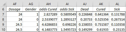 Figure 6 – Forecasted probabilities
From Figure 6, we see that the multinomial logistic regression model described on this webpage forecasts that 22.7% of women who receive a dosage of 24 mg will die, 64.1% will be cured and 13.2% will be sick. This compares with 12/63 = 19% of the sample women who receive a dosage will die, 15/63 = 24% who will be cured and 36/63 = 57% who will be sick. Even though we have no sample data for 24.5 mg the model produces the forecast shown in Figure 6.
The following formulas are used to create the first row of data in Figure 6:
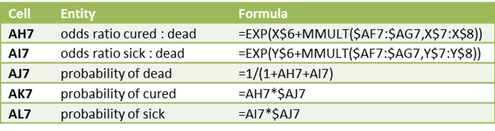 Figure 7 – Key formulas for Figure 6
Good morning Charles,
just for confirmation the coefficients were calculated using solver right?
But my answer ins slightly different.
Harissa,
These coefficients could also be calculated using Newton’s method.
Charles
Dear Charles,
I am greatly thankful to you for this wonderful tool.
I want to know if there is any method or functions on “how to find out the intercept and coefficients of the reference outcome i.e. Dead” from the examples.
Thanks again
Thank you for your honourable contribution the advancement of knowledge. Please, I implore you to act fast in line with William Agurto’s observation.
Hello,
Thanks for your input.
The multinomial logistic regression data analysis tool is already part of the Real Statistics software. I still need to implement the ordinal logistic regression tool.
Charles
Hi Charles,
I don’t follow on this statement:
“That exp(bgender) = 1.116 for Cured + Dead means that for any given dosage women are 11.5% more likely than men to be cured rather than dead. ”
Where does the 11.5% come from?
Alan,
I believe that it is a typo and should be 11.6% (i.e. 1.116-1 = .116).
Thanks for finding this typo.
Charles
Hi Charles,
I calculated the coefficients for the cured +dead model using the LogitCoeff function just to see is there were any differences. The LogitCoeff function changes the signs for of the coefficients. Why would that be?
Hi Marc,
Are you referring to MLogitCoeff or LogitCoeff? If the latter, what are specific arguments are you using?
Charles
Hi Charles,
I am trying to use your tool for Multiple logistic regression (by Ctrl +m) but when i get an error saying : “Alpha must be between 0 and 0.5” although i leave at the default value of 0.05. I have tried multiple values within this range to no success. Not sure why i get this error..
Thanks
Dimitris
Hi,
This is a problem related to how your version of Excel interprets decimals (comma rather than period). I suggest that you simply re-enter the value for alpha using whatever version of the decimal symbol you normally use. Don’t use the default (even if it is identical to what you enter).
Charles
Dear Charles,
Thank you so much for your help. I didn’t understand “1.0” and “2.0” in the formula(=+LogitCoeff(MLogitExtract(A5:E16;2;”1,0″;FALSE))). And I kindly ask you if it means :
Dead = “0”
Cured=”1,0″
Sick=”2,0″
?
If it were binary logistic regression modelling, would it be only “1,0” ?
The other question is that, by selecting A5:E16, how does the formula separates the independents from the dependents?
Thank you very much
MLogitExtract(A5:E16;2;”1,0″;FALSE) is a data range that is used as the input to the LogitCoeff function (caution: the formula you have written has an extra right parenthesis). The resulting data range is derived from the original data range A5:E16 (the first argument in the function). Since the second argument in the function is 2, we know that the last three columns of the original data range correspond to the dependent variables 0, 1, 2. Since A5:E16 has 5 columns, this means that the first two columns correspond to the two independent variables and the last three columns correspond to the three dependent variables.
The output from the MLogitExtract will always have the exact same independent variables as found in original data range (i.e. columns A and B for the example). Only the dependent variable may change (i.e. which variables are retained and potentially the order of these variables), this is determined by the third argument: “1,0” in the example. Here “1,0” means that you should retain dependent variables 1 (i.e. Cured) followed by 0 i.e. Dead). Thus the output from MLogitExtract(A5:E16;2;”1,0″;FALSE) is equivalent to column A, followed by column B, followed by column D followed by column C; i.e. columns C and D are interchanged and column E is not used.
The output from MLogitExtract(A5:E16;2;”0″;FALSE) would consist of columns A through C. Dead would then be the only dependent variable (binary logistic regression).
The output from MLogitExtract(A5:E16;2;”2,0″;FALSE) would consist of columns A, B, E, C, that order. Sick and Dead would then be the only dependent variables.
Charles
Dear Charles:
Although the methods to calculate coefficients for multiple logistic regression and ordinal logistic regression are well explained, following those steps become tedious and impractical when there are many independent and dependent variables. Is it possible to develop an add-in that totally and directly solves multiple logistic regression and ordinal logistic regression, without the use of binary logistic regression as an intermediate way (because this needs entering additional formulas by the user)?
Thank a lot.
William Agurto.
William,
I agree. These are on my things to do list.
Charles