Principal component analysis is a statistical technique that is used to analyze the interrelationships among a large number of variables and to explain these variables in terms of a smaller number of variables, called principal components, with a minimum loss of information.
Definition 1: Let X = [xi] be any k × 1 random vector. We now define a k × 1 vector Y = [yi], where for each i the ith principal component of X is
![]()
for some regression coefficients βij. Since each yi is a linear combination of the xj, Y is a random vector.
Now define the k × k coefficient matrix β = [βij] whose rows are the 1 × k vectors 
yi = 
For reasons that will be become apparent shortly, we choose to view the rows of β as column vectors βi, and so the rows themselves are the transpose
Observation: Let Σ = [σij] be the k × k population covariance matrix for X. Then the covariance matrix for Y is given by
ΣY = βT Σ β
i.e. population variances and covariances of the yi are given by
![]()
![]()
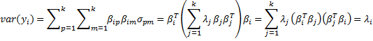
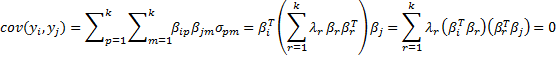
Observation: Our objective is to choose values for the regression coefficients βij so as to maximize var(yi) subject to the constraint that cov(yi, yj) = 0 for all i ≠ j. We find such coefficients βij using the Spectral Decomposition Theorem (Theorem 1 of Linear Algebra Background). Since the covariance matrix is symmetric, by Theorem 1 of Symmetric Matrices, it follows that
Σ = β D βT
where β is a k × k matrix whose columns are unit eigenvectors β1, …, βk corresponding to the eigenvalues λ1, …, λk of Σ and D is the k × k diagonal matrix whose main diagonal consists of λ1, …, λk. Alternatively, the spectral theorem can be expressed as

Property 1: If λ1 ≥ … ≥ λk are the eigenvalues of Σ with corresponding unit eigenvectors β1, …, βk, then
and furthermore, for all i and j ≠ i
var(yi) = λi cov(yi, yj) = 0
Proof: The first statement results from Theorem 1 Symmetric Matrices as explained above. Since the column vectors βj are orthonormal, βi · βj = 
Property 2:
![]()
Proof: By definition of the covariance matrix, the main diagonal of Σ contains the values 


Observation: Thus the total variance
Thus the portion of the total variance (of X or Y) explained by the ith principal component yi is λi/
Our goal is to find a reduced number of principal components that can explain most of the total variance, i.e. we seek a value of m that is as low as possible but such that the ratio
Observation: Since the population covariance Σ is unknown, we will use the sample covariance matrix S as an estimate and proceed as above using S in place of Σ. Recall that S is given by the formula:
![]()
where we now consider X = [xij] to be a k × n matrix such that for each i, {xij: 1 ≤ j ≤ n} is a random sample for random variable xi. Since the sample covariance matrix is symmetric, there is a similar spectral decomposition

where the Bj = [bij] are the unit eigenvectors of S corresponding to the eigenvalues λj of S (actually this is a bit of an abuse of notation since these λj are not the same as the eigenvalues of Σ).
We now use bij as the regression coefficients and so have
![]()
and as above, for all i and j ≠ i
var(yi) = λi cov(yi, yj) = 0
![]()
As before, assuming that λ1 ≥ … ≥ λk, we want to find a value of m so that
Example 1: The school system of a major city wanted to determine the characteristics of a great teacher, and so they asked 120 students to rate the importance of each of the following 9 criteria using a Likert scale of 1 to 10 with 10 representing that a particular characteristic is extremely important and 1 representing that the characteristic is not important.
- Setting high expectations for the students
- Entertaining
- Able to communicate effectively
- Having expertise in their subject
- Able to motivate
- Caring
- Charismatic
- Having a passion for teaching
- Friendly and easy-going
Figure 1 shows the scores from the first 10 students in the sample and Figure 2 shows some descriptive statistics about the entire 120 person sample.

Figure 1 – Teacher evaluation scores

Figure 2 – Descriptive statistics for teacher evaluations
The sample covariance matrix S is shown in Figure 3 and can be calculated directly as
=MMULT(TRANSPOSE(B4:J123-B126:J126),B4:J123-B126;J126)/(COUNT(B4:B123)-1)
Here B4:J123 is the range containing all the evaluation scores and B126:J126 is the range containing the means for each criterion. Alternatively, we can simply use the Real Statistics formula COV(B4:J123) to produce the same result.

Figure 3 – Covariance Matrix
In practice, we usually prefer to standardize the sample scores. This will make the weights of the nine criteria equal. This is equivalent to using the correlation matrix. Let R = [rij] where rij is the correlation between xi and xj, i.e.
![]()
The sample correlation matrix R is shown in Figure 4 and can be calculated directly as
=MMULT(TRANSPOSE((B4:J123-B126:J126)/B127:J127),(B4:J123-B126:J126)/B127:J127)/(COUNT(B4:B123)-1)
Here B127:J127 is the range containing the standard deviations for each criterion. Alternatively, we can simply use the Real Statistics function CORR(B4:J123) to produce the same result.

Figure 4 – Correlation Matrix
Note that all the values on the main diagonal are 1, as we would expect since the variances have been standardized. We next calculate the eigenvalues for the correlation matrix using the Real Statistics eigVECTSym(M4:U12) formula, as described in Linear Algebra Background. The result appears in range M18:U27 of Figure 5.

Figure 5 – Eigenvalues and eigenvectors of the correlation matrix
The first row in Figure 5 contains the eigenvalues for the correlation matrix in Figure 4. Below each eigenvalue is a corresponding unit eigenvector. E.g. the largest eigenvalue is λ1 = 2.880437. Corresponding to this eigenvalue is the 9 × 1 column eigenvector B1 whose elements are 0.108673, -0.41156, etc.
As we described above, coefficients of the eigenvectors serve as the regression coefficients of the 9 principal components. For example, the first principal component can be expressed by
![]() This can also be expressed as
This can also be expressed as
![]()
Thus for any set of scores (for the xj) you can calculate each of the corresponding principal components. Keep in mind that you need to standardize the values of the xj first since this is how the correlation matrix was obtained. For the first sample (row 4 of Figure 1), we can calculate the nine principal components using the matrix equation Y = BX′ as shown in Figure 6.

Figure 6 – Calculation of PC1 for first sample
Here B (range AI61:AQ69) is the set of eigenvectors from Figure 5, X (range AS61:AS69) is simply the transpose of row 4 from Figure 1, X′ (range AU61:AU69) standardizes the scores in X (e.g. cell AU61 contains the formula =STANDARDIZE(AS61, B126, B127), referring to Figure 2) and Y (range AW61:AW69) is calculated by the formula
=MMULT(TRANSPOSE(AI61:AQ69),AU61:AU69)
Thus the principal component values corresponding to the first sample are 0.782502 (PC1), -1.9758 (PC2), etc.
As observed previously, the total variance for the nine random variables is 9 (since the variance was standardized to 1 in the correlation matrix), which is, as expected, equal to the sum of the nine eigenvalues listed in Figure 5. In fact, in Figure 7 we list the eigenvalues in decreasing order and show the percentage of the total variance accounted for by that eigenvalue.

Figure 7 – Variance accounted for by each eigenvalue
The values in column M are simply the eigenvalues listed in the first row of Figure 5, with cell M41 containing the formula =SUM(M32:M40) and producing the value 9 as expected. Each cell in column N contains the percentage of the variance accounted for by the corresponding eigenvalue. E.g. cell N32 contains the formula =M32/M41, and so we see that 32% of the total variance is accounted for by the largest eigenvalue. Column O simply contains the cumulative weights, and so we see that the first four eigenvalues account for 72.3% of the variance.
Using Excel’s charting capability, we can plot the values in column N of Figure 7 to obtain a graphical representation, called a scree plot.

Figure 8 – Scree Plot
We decide to retain the first four eigenvalues, which explain 72.3% of the variance. In section Basic Concepts of Factor Analysis we will explain in more detail how to determine how many eigenvalues to retain. The portion of Figure 5 that refers to these eigenvalues is shown in Figure 9. Since all but the Expect value for PC1 is negative, we first decide to negate all the values. This is not a problem since the negative of a unit eigenvector is also a unit eigenvector.
")
Figure 9 – Principal component coefficients (Reduced Model)
Those values that are sufficiently large, i.e. the values that show a high correlation between the principal components and the (standardized) original variables, are highlighted. We use a threshold of ±0.4 for this purpose.
This is done by highlighting the range R32:U40 and selecting Home > Styles|Conditional Formatting and then choosing Highlight Cell Rules > Greater Than and inserting the value .4 and then selecting Home > Styles|Conditional Formatting and then choosing Highlight Cell Rules > Less Than and inserting the value -.4.
Note that Entertainment, Communications, Charisma and Passion are highly correlated with PC1, Motivation and Caring are highly correlated with PC3 and Expertise is highly correlated with PC4. Also, Expectation is highly positively correlated with PC2 while Friendly is negatively correlated with PC2.
Ideally, we would like to see that each variable is highly correlated with only one principal component. As we can see from Figure 9, this is the case in our example. Usually, this is not the case, however, and we will show what to do about this in the Basic Concepts of Factor Analysis when we discuss rotation in Factor Analysis.
In our analysis, we retain 4 of the 9 principal factors. As noted previously, each of the principal components can be calculated by
![]() i.e. Y= BTX′, where Y is a k × 1 vector of principal components, B is a k x k matrix (whose columns are the unit eigenvectors) and X′ is a k × 1 vector of the standardized scores for the original variables.
i.e. Y= BTX′, where Y is a k × 1 vector of principal components, B is a k x k matrix (whose columns are the unit eigenvectors) and X′ is a k × 1 vector of the standardized scores for the original variables.
If we retain only m principal components, then Y = BTX where Y is an m × 1 vector, B is a k × m matrix (consisting of the m unit eigenvectors corresponding to the m largest eigenvalues) and X′ is the k × 1 vector of standardized scores as before. The interesting thing is that if Y is known we can calculate estimates for standardized values for X using the fact that X′ = BBTX’ = B(BTX′) = BY (since B is an orthogonal matrix, and so, BBT = I). From X′ it is then easy to calculate X.

Figure 10 – Estimate of original scores using reduced model
In Figure 10 we show how this is done using the four principal components that we calculated from the first sample in Figure 6. B (range AN74;AQ82) is the reduced set of coefficients (Figure 9), Y (range AS74:AS77) are the principal components as calculated in Figure 6, X′ are the estimated standardized values for the first sample (range AU74:AU82) using the formula =MMULT(AN74:AQ82,AS74:AS77) and finally, X are the estimated scores in the first sample (range AW74:AW82) using the formula =AU74:AU82*TRANSPOSE(B127:J127)+TRANSPOSE(B126:J126).
As you can see the values for X in Figure 10 are similar, but not exactly the same as the values for X in Figure 6, demonstrating both the effectiveness as well as the limitations of the reduced principal component model (at least for this sample data).
Hello Charles. Thanks very much for this tool. I am trying to do a principal component analysis across 34 countries. I have three variables currently (disclosure, burden of proof, and anti director right) and I want to use PCA to create a new variable called insider protection which is a PCA of these three variables. The output should be an index number for each of the 34 countries. I am running into a few issues: 1) I don’t know the best way to set up the data (i.e. countries as rows vs. columns) and 2) Even if I try the set up both ways I get more eigenvectors than variables. I have the Excel file, just not sure how to send it to you.
Hello Kamini,
I have now received your email with the Excel attachment. I will look at it shortly.
Charles
Charles,
Thank you so much for such valuable tool! I had a question: when I calculate the eigenvalues and eigenvectors, the vector have more coefficients than I have variables in the dataset. Any idea why this is happening?
Thanks again for this amazing tool!
Hello Federico,
If you email me an Excel spreadsheet with your data and results, I will try to figure out why this is happening.
Charles
I often see PCA score plots in the literature, with PC1 on the x-axis and PC2 on the y-axis showing a cloud of dots. I assume the PC1 scores were generated as the sum of the eigenvector coefficients of the largest eigenvalue multiplied by the corresponding original values. This value would be -12.6 for student 1. The PC2 scores use the eigenvector coefficients of the next largest eigenvalue applied to the original values. If this is not the case I would appreciate knowing how to interpret the PCA score plots. Thanks.
Hi Dave,
Without seeing your data and analysis, I am not able to address your comment.
Charles
Hi Charles,
I had attempted for PCA using real stat functions as depicted,
however I am getting eigen vector with sign reversed for eigen vector/ PC 1,2,4,5 and 7.
further, comparison of eigen vector in demo and in Minitab indicates sign reversed for eigen vector/PC 1,4 and 7.
Can you help to understand possible reason for this, and how do I get similar PC using Real Stats and Minitab.
Thanks!
Hello,
It is not a problem if all the signs of the eigenvectors are reversed. This is normal. Remember that eigenvectors are not unique. In fact, if X is an eigenvector then so is -X.
Charles
Hello Charles, Thanks for illustration on PCA using Excel.
Can you share the excel with with raw data (with 120 observations) and analysis completed, shown step wise.
You can download the spreadsheet that performs PCA for the problem on this webpage. Just download the Multivariate Analysis examples workbook from https://www.real-statistics.com/free-download/real-statistics-examples-workbook/
Charles
Hi Charles,
Thank you for detailed explaination about PCA.
I downloaded the data from Multivariate Analysis examples workbook.
But it seems wrong data.
—————
Multivariate Real Statistics Using Excel – Examples Workbook
Charles Zaiontz, 13 April 2021
Copyright © 2013 – 2021 Charles Zaiontz
——————–
Could you please show where to download the data.
Thank you
Nguyen Thang
Hi Charles
I have found the data for PCA.
That’s great.
Thank you
Hi Mr, Zaiontz
I really appreciate your site. Many thanks
Also, i want to ask you about how can I performance a PCA with covariance matrix?
I’was practicing but I just get correlation matrix.
Thanks in advance,
Best regards, Max
Hi Max,
Is there any particular reason for using the covariance matrix instead of the correlation matrix?
I believe that the process is similar, but I always use the correlation matrix.
Charles
Thanks for answering me Mr. Charles
Yes, the point is that I am seeing the benefits of both methods, that is, the differences in the results to understand the values obtained well, and then try the most robust versions of pca, on a non-Gaussian, non-linear database , with outliers and of very high dimension, as a geological database
Thank you very very much
Hello Charles,
Thanks a lot for the article. I was just wondering how can we calculate the expected values for the other samples (e.g., 2, 3, 4…), other than the first one (as you did on figure 10, column “AW”), using the computed PCs.
Leonardo,
This is done in exactly the same way.
Charles
Hello dear Charles, I have tried follow your explanation about using formulas eValues in Excel, unfortunately it does not exists in my tool pack, what should I do, thank you in advance
Gilad,
You need to download and install the Real Statistics tool pack to use this and many other capabilities. You can download this tool pack for free from https://www.real-statistics.com/free-download/real-statistics-resource-pack/
Charles
Hi Charles,
I’ve followed all the theoretical explaination, the only things i’m in trouble with is concrete use XRealstat’s formula:
Do you know why if I put these formula (as you did in the example) COV(…) you have had a matrix and i’ll recived back just a cell with a single number ??
It’s going on with all the types of formula.
Really thanks for your support!!
Toto,
This problem occurs because COV and many other functions are what Microsoft calls array functions. These need to be handled in a slightly different way. See the following webpage:
Array Formulas and Functions
Charles
Really Thanks Charles,
you’ve now filled my gap!
Hey Charles,
The file THC.csv contains data on concentrations of 13 different chemical compounds in marijuana plants own in the same region in Colombia that are derived from three different species varieties. I was performing PCA where in i was stuck here. Could you please help me Perform a principal component analysis using SAS on the correlation matrix and answer the following questions from the resultant SAS output.
1. Obtain the score plot of PC 2 versus PC1. Is there any discernable outliers or pattern that you can comment on?
2. Obtain the score plot of PC 2 versus PC1 using the covariance matrix. Are there any discernable outliers or pattern that you can comment on?
3. Obtain the score plot of PC 2 versus PC1 using the correlation matrix. Are there any discernable outliers or pattern that you can comment on?
4. Obtain the score plot of PC 2 versus PC1 using the standardized PCs. Are there any discernable outliers or pattern that you can comment on?
5. Find the 95% confidence intervals for the first to fifth eigenvalues.
Thanks,
Lakshmi
Sorry, but I don’t use SAS. This website explains how to perform PCA in Excel.
Charles
Hello Charles,
When I run eVectors, it generates two additional rows at the bottom that are not discussed here. So, when I input, say, a 5×5 matrix, the output is 8×5 but my understanding is that the output should be a 6×5 matrix. I’ve tried using the formula in your sample Excel sheet for the exact dataset used in the example and it still occurs. However, up until that point, the results of the matrices are identical.
Thank you,
Nicole
Nicole,
These last two rows can be used to detect errors. They are not part of the eigenvalues/eigenvectors results. See
https://real-statistics.com/linear-algebra-matrix-topics/eigenvalues-eigenvectors/
https://real-statistics.com/linear-algebra-matrix-topics/eigenvectors-for-non-symmetric-matrices/
Charles
Why does the PC1 column flips its pos/neg sign between Fig 5 & 9?
Kris,
If X is an eigenvector for eigenvalue c, then so is -X. I tend to use the sign that results in the fewer negative values.
Charles
I tried using the direct calculations for the covariance & correlation matrices, but they do not produce the same results at the COR and COV functions in the add-in. Am I missing something?
Hello Kris,
They should produce the same results. If you email me an Excel file with your data and results, I will try to figure out what is going wrong.
Charles
Hi Charles,
I have a data matrix of 35 samples and 255 observations. The final Eigenvector calculation results is a matrix 256×255. How long should the calculation take. It’s been running for two hours and is not finished.
Thanks
Ilan
Hi Ilan,
I haven’t optimized the eVECTORS function for speed and don’t know how long it should take. In any case, I have the following suggestion that will likely reduce the time it takes considerably:
The second argument in the eVECTORS function is the # of iterations used. This defaults to 100. This number is very likely to be much higher than you need. I suggest that you use a much smaller value, say 10. I suggest that you highlight an output range with two extra rows. If the first of these rows is all zeros, then you know that the calculated eigenvalues are correct, while if the second of these rows is all zeros then you know that the calculated eigenvectors are correct (and so you used a sufficient number of iterations).
Charles
Hi Charles I am not able to use these formulas directly in my data. I have tried many ways but couldn’t. Is there any way to do, or I have to do it step wise.
MMULT(TRANSPOSE(B4:J123-B126:J126),B4:J123-B126;J126)/(COUNT(B4:B123)-1)
Hello,
This is an array formula and so you can’t simply press Enter. See
Array Formulas and Functions
Charles
Dear Charles,
I tried PCA again. The results are amazing. Beyond intuition.
It is showing 79th teacher is the best though sum of his scores are lowest (33). Maybe because his scores are highest in EXPECT and PCA places highest emphasis on EXPECT.
Here is list of top-10 teachers by score. Please correct me if I am wrong.
Thanks
balnagendra
sno expect entertain comm expert motivate caring charisma passion friendly score
79 4.37 -0.06 0.85 1.61 1.16 1.53 -0.13 0.61 0.27 10.22
76 2.40 -0.24 0.54 1.96 0.54 -0.05 0.89 0.21 0.65 6.88
13 3.59 1.89 0.31 0.15 1.04 0.50 -0.26 -0.47 -0.03 6.72
22 1.39 1.08 1.65 0.89 -0.01 1.14 -0.25 -0.31 0.66 6.24
7 1.17 0.37 1.11 1.57 0.63 0.19 -0.07 0.13 0.04 5.14
87 3.70 0.74 0.70 -0.19 -0.37 0.17 -0.65 0.38 0.32 4.81
102 1.46 1.28 0.99 0.27 -0.54 0.21 0.63 0.16 -0.18 4.28
71 -0.02 1.96 1.10 -0.23 -0.09 1.04 0.22 0.08 0.21 4.26
80 0.32 1.02 0.35 0.26 0.44 -0.02 0.81 0.34 0.40 3.91
56 1.33 0.12 0.55 0.15 1.04 0.58 0.66 -0.29 -0.43 3.71
91 1.75 0.68 1.12 1.41 -0.59 -0.42 -0.11 0.28 -0.49 3.63
Glad to see that you got it to work. Sorry, but I don’t have the time to check your work about the top teachers.
CHarles
Im getting this as top 10 since only pc1..pc4 are taken into consideration.
sr
16 2.24 2.36 1.27 3.97
13 3.59 1.89 0.31 -0.15
87 3.70 0.74 0.70 0.19
120 2.39 -0.64 1.28 2.01
40 1.43 1.33 1.30 -0.49
79 4.37 -0.06 0.85 -1.61
51 2.08 -0.19 0.10 1.51
102 1.46 1.28 0.99 -0.27
71 -0.02 1.96 1.10 0.23
22 1.39 1.08 1.65 -0.89
now ambiguity is going to lead to confusion…. hope charles comes for rescue.
many thanks
Hi, Charlie
I downloaded the add-in, and it works to calculate CORR and COV. But eVectors() returns all 0. No clue what the problem is. Any suggestion ?
Thanks.
Yong
Hello Yong,
I introduced a bug in Rel 7.0. I will correct this later today with Rel 7.0.1
Charles
Thanks, Charles
A silly question: We usually calculate the eigen-values and vectors from CORR matrix, and apply {s} to eigen vector to get the real magnitude. eVectors can be applied to COV matrix too and it returns another set of eigen values and vectors. Are they easily convertible to the eigen results from CORR matrix ? Or, are the results from COV usable ?
Hi ,
Ive used MEigenvalPow , MEigenvec to find the vectors from the add in… whilst using eigenvalPow make sure you select only 1 row as output row 1×9, and use it as an array function.
Hope it helps
Hi. I have a time series of yield curve constituents (i.e. 2y-30y). How this changes the methodology? I have constructed the standardized correl matrix and estimated the eigenvalues and vector. How should I proceed from there? In your example you have 10 students with 10 response categories. I have 5y monthly data for 10 bond yields.
The approach should be the same, but I don’t know whether PCA is an appropriate approach. What are you trying to accomplish?
Charles
Hi Charles, thank you for your PCA calculation example. It is quite useful and the procedure makes sense. I was wondering if you could show me how to apply the same methodology to a large sample. You showed us how to calculate the principal components for the first sample. Can you show me the formulas for calculating the principal components for the entire sample in one matrix iteration. Or do I have to calculate them individually for each sample. Thanks.
Hello Massoud,
The approach described also works for a large sample.
Are you trying to apply the PCA approach for multiple samples? If so, you need to repeat the approach for each sample.
Charles
Got it. Thanks so much for the quick reply.
Hi Charles,
Thank you very much for this instructive website and resource.
I understand it that the values you calculated for the first sample (“Y”, AW61:AW69) in Fig 6 are the coordinates that can be used in a PCA dot plot of the kind that is most commonly presented for identifying eg subgroups within a population with the aid of PCA (eg https://miro.medium.com/max/1200/1*oSOHZMoS-ZfmuAWiF8jY8Q.png).
My guess is that one chooses the two “top” PCs in a 2-D plot and the top 3 in a 3-D plot. That would correspond to cells AW61:AW62 or AW61:AW63 in Fig 6, respectively.
Are the above assumptions correct?
Best,
Dan
Hello Dan,
There are many opinions as to which PCs to retain, most commonly via the scree plot. I guess by definition for a 2D plot you would choose the top two and for a 3D plot you would choose the top three.
Charles
Ah, misunderstanding.
My question was this: In the type of plot I was linking to, individual data points are shown as points in a space determined by the two or three PCs with highest eigenvalues. The actual coordinates of those points in the PC space, are those the values found in column AW in Fig 6? Or should those coordinates be calculated by a different method?
It seems to me that the relative magnitude of the eigenvalues are not accounted for in the column AW values, so that the “swarm” of points appears to extend equally far in all PC directions. That would be misleading, wouldn’t it? I would imagine that instead of multiplying with AI61:AQ69, a matrix consisting of the eigenvector coordinates _multiplied by their respective eigenvalues_ should be used. But I am only guessing here. What do you say?
Hi Dan,
Assuming for a moment that you have two PC’s, are you trying to create a two-dimensional plot of the original data in this two-dimensional space?
Charles
Let’s say that. It could be a 3-D plot. It is not important, but let’s take 2-D. My question is: are the coordinates for the first data point in such a plot to be found in cells AW61:AW62 (or in AW61:AW63 for a 3-D plot)?
Hello Dan,
I am still trying to understand what you are trying to plot. Are you trying to plot the original data transformed into the two or three dimensions defined by the principal component analysis (assuming two or three PCs are retained)?
Charles
In reply to the question: “Are you trying to plot the original data transformed into the two or three dimensions defined by the principal component analysis (assuming two or three PCs are retained)?”
The answer to that is yes.
Dan,
In the example shown on the webpage, the 9 coordinates for each data element are mapped into 4 coordinates since 4 principal components are retained in the reduced model. (I believe that for your example, you will retain either 2 or 3 principal components instead of 4). Figure 6 shows the mapping of the 9 coordinates for the first data element into 9 PC coordinates. Since only 4 PCs are retained in the reduced model, I believe that you would retain only the first 4 of these coordinates, i.e. (.78, -1.97, -.23, 1.12). If your model retains only two PC’s, then the first two coordinates become the values that you would plot on the chart.
The situation is a bit more complicated for the PC version of Factor Analysis, where factor scores are used. This is explained on the following webpage:
Factor Scores
(see, for example, Figure 1).
Charles
Thank you very much. I am still a bit puzzled about how best to plot these values. The values in column AW of Fig 6 are standardised, as I understand it, meaning that regardless of the actual variance in the original data, they will be spread out equally in their respective PC dimensions. Right? If so, then it would not be discernible from such a plot which PC is responsible for which proportion of the variance. Isn’t that a drawback?
And could one not use another eigenvector matrix to generate the data for the plot, where the magnitudes of the respective eigenvalues are accounted for as well?
Hello Dan,
The following webpage may clarify things. See, especially, the orthogonal rotation plot
https://stats.idre.ucla.edu/spss/seminars/introduction-to-factor-analysis/a-practical-introduction-to-factor-analysis/
Charles
I’m trying to teach myself PCA, and I would like to work your example out. Could you provide the entire original data set (all 120 students’ teacher ratings)? Thanks.
Hello John,
You can download this at Real Statistics Examples Workbooks.
Charles
Hello John,
You can download this at https://real-statistics.com/free-download/real-statistics-examples-workbook/
Charles
John,
The PCA example is located in the Multivariate Examples workbook.
Hi Charles,
Great example but I still do not understand what’s the final criteria of being a good teacher and the level of significance for each criteria based on your results. What I’m getting at basically is, if I want to use the results of the PCA as a weighing factor for each variable, how should I do it? What I mean by that is which of the characteristic should be chosen as final determinants/criteria of a good teacher and how much weight can be associated to each of the determinant based on the result of the PCA?
Hello Dante,
I believe that you are referring to the factor scores as described at
https://real-statistics.com/multivariate-statistics/factor-analysis/factor-scores/
Charles
Can any variable be run on PCA? Like i have 8 variables namely Time of the day (1-24), day of the week (1-7) Month of the year (1-12) Working Day or Not (1 or 0) Actual Demand (in Megawatts), Average temperature (deg Celcius), Percent Humidity and Average Rainfall (mm). My data set is from January 1, 2012 to December 25, 2017. There are 52,465 rows of data since it is in hourly basis. Can i run all of theses in PCA?
Hi Ricmart,
Yes, you should be able to use any of these variables by using the specified coding.
Charles
Dear Charles,
I performed 50 number of tests and calculated Mean, Median, Skew, Kurtosis, relevant x values for Probabilities of 1%, 2%,5%,10%,50% using WEIBULL_INV(p, β, α) and Normal inverse functions for each test. Can I use PCA for reducing these data to one or two variables for comparison?
Umesh,
Interesting idea. You can certainly perform PCA. I don’t know whether the results will be that useful, but you should try and see what happens.
Charles
Thank you for your very helpful website!
Hi Charles,
Thanks for this article, could you explain a bit about bellow mentioned, I am quoting you here:
Statment 1:”Alternatively we can simply use the Real Statistics formula COV(B4:J123) to produce the same result”
My Understanding: It will produce covariance matrix of original data ranges (B4:J123)
Statment 2: “Alternatively we can simply use the Real Statistics function CORR(B4:J123) to produce the same result”
My Understanding : It will produce corelation matrix of my original data ranges (B4:J123)
Statment 3: “We next calculate the eigenvalues for the correlation matrix using the Real Statistics eVECTORS(M4:U12) formula, as described in Linear Algebra Background. The result appears in range M18:U27 of Figure 5.”
My Understanding: Calculate the eigen vector based on the corellation matrix which we obtained from statment 2 above and result is in M18:U27
Statment 4: “Keep in mind that you need to standardize the values of the xj first since this is how the correlation matrix was obtained”
My Understanding : CONFUSED !!
Where did we standardise our intial data? the ‘xj’s here, we obtain both corelation and covariance matrix based on our original data that is ranges in B4:J123
I know standardisation is required for PCA, but our operations of calculating eigenvactors etc. is based on corelation matrix which we obtained from corelation matrix calculated on our orginal data. So what is the point of covariance matrix or whats the use of the same.
This is what you mentioned after we got the corelation matrix, but where did we standardize our data ? This corealtion matrix is based on our original data set.
“Note that all the values on the main diagonal are 1, as we would expect since the variances have been standardized”
Hope you clarify
Udayan,
Standardizing the data will result in a covariance matrix that has ones on the main diagonal. You get the same answer if instead of standardizing the data you use the correlation matrix (on the original data) instead of the covariance matrix.
Charles
You say that ideally, we want to have each variable to highly correlated with only one principal component and that we will see that in the rotation section of factor analysis. But there, you apply the rotation to the first 4 column of the load matrix. Here we are interested in the eigen vectors and eigen values matrix. Can we apply the rotation, for example varimax, to the first four columns of this matrix as well?
Olivier,
Sorry, but I don’t understand your question. Varimax is used to rotate a matrix. Are you referring to a different matrix?
Charles
Here, for the principal component; you consider the matrix in figure 9. I quote you about the interpretation of the results “Ideally we would like to see that each variable is highly correlated with only one principal component. As we can see form Figure 9, this is the case in our example. Usually this is not the case, however, and we will show what to do about this in the Basic Concepts of Factor Analysis when we discuss rotation in Factor Analysis.” But in the factor analysis section, you rotate another matrix, not the one in figure 9 and this is also what the tool in the analysis toolpack do. My question is then, should we apply the rotation (for example varimax) to the matrix in figure 9? I understand that it will “work” in the sense that it is defined. But does it make sense to do so? Does it fit to the model; which resemble, but is not exactly the same as the one in the factor analysis? Would this return “Principal Component” that highly correlate with only one variable?
Olivier,
Thanks for the clarification. I now understand your question. I will try to answer your question shortly, but I need to first finish up some other things that I am working on.
Charles
Olivier,
See the following webpage:
https://stats.stackexchange.com/questions/612/is-pca-followed-by-a-rotation-such-as-varimax-still-pca
Charles
hi, great site and I like that you answer to our questions in a dedicated way and fast…The question I’d like to ask is what is the correlation of regression and PCA.
From my understanding the correlations of a factor and its constituent variables is a form of linear regression – multiplying the x-values with estimated coefficients produces the factor’s values
And my most important question is can you perform (not necessarily linear) regression by estimating coefficients for *the factors* that have their own now constant coefficients)
hi, I also wanted to ask was
with is the difference between eigenvectors calculated from correlation matrix and eigenvectors calculated with covariance matrix?how are they different? for what purpose is each better suitable for?
Savvas,
The eigenvalues as well as the eigenvectors for the correlation and covariance matrices will be different. I have not investigated whether there is any relationship between them. Perhaps the following webpage will address your last question:
https://stats.stackexchange.com/questions/53/pca-on-correlation-or-covariance
Charles
Thanks for this! The breakdown through Excel helped me understand PCA a lot better.
I’ve followed the accompanying workbook and I think there might be an error in the multivariate workbook in the PCA tab, AS61 to AS69 as it just picks up the first row in the raw data. Am I right in saying so?
Cheers.
Bea,
I am pleased that this webpage helped you understand PCA better.
The range AS61:AS69 is only intended to show the first row in the raw data, as explained in Figure 6 of the webpage.
Charles
Hello Charles,
I hope you are well! When you say:
“Observation: Our objective is to choose values for the regression coefficients βij so as to maximize var(yi) subject to the constraint that cov(yi, yj) = 0 for all i ≠ j. We find such coefficients βij using the Spectral Decomposition Theorem (Theorem 1 of Linear Algebra Background). Since the covariance matrix is symmetric, by Theorem 1 of Symmetric Matrices, it follows that
Σ = β D βT
where β is a k × k matrix whose columns are unit eigenvectors β1, …, βk corresponding to the eigenvalues λ1, …, λk of Σ and D is the k × k diagonal matrix whose main diagonal consists of λ1, …, λk. Alternatively, the spectral theorem can be …”
Do you mean Σy? Are we decomposing X’s covariance matrix or Y’s?
Sorry, I think I got confused about that part.
Thanks in advance!
Fred
Oooooops, sorry, it actually makes sense now…very nice… the betas cancel out and still the variance is maximised and the covariance minimised. This is actually one of those moments where maths are beautiful 🙂
Is there a geometric interpretation of the process? It is almost like using an eigenvector basis that captures more variance than the standard basis…
Once again, superb explanation!!!
Thanks Charles
Fred,
The geometric interpretation related to an orthogonal transformation. See the following for more information:
http://cda.psych.uiuc.edu/kelley_handout.pdf
Charles
Hi I get a single cell answer when I use eVectors function on a 8×8 correlation matrix. Why is this?
Omachi,
eVectors is an array function and so you can’t simply press Enter when you use this function. See the following:
Array Functions and Formulas
Charles
in defn 1 shouldnt Y = beta*X and not beta^T*X also where does beta^T*X=[beta(i,j)] come from none of this seems clear.
Brian,
Since beta is a k x k matrix, it really doesn’t matter whether we view Y = beta x X or Y = beta^T x X, as long as we are consistent.
For any row i, beta_i^T is a k x 1 column vector whose values are the beta_ij values for the given i.
I agree that the notation is a bit confusing. It is probably easier to following things using the real example that is described on the webpage.
Charles
Dear Charles,
Thanks for your website.
I have done PCA calculation inch-by-inch on teachers data with a mix of R, Excel and now RDBMS.
Here are the final results by sample sno.
I have two questions:
1. What after this. Which sample is the best fit.
Like in Heptathlon example who becomes the winner.
How do I calculate the final winner.
What if final results do not match PCA scores.
What I understood by PCA analysis it is telling me which attributes are important as per the student samples.
Hence the name Principal Component Analysis.
Can this tell me which student did the best analysis?
2. It is though a trivial question, why do I have to reduce 9 dimensions to 4 only.
Because with RDBMS coming into picture it takes no extra effort to calculate all 9 dimensions.
thanks and regards
Balnagendra
“sno” “pc1” “pc2” “pc3” “pc4” “pc5” “pc6” “pc7” “pc8” “pc9”
1 0.782502087334704 -1.96757592201719 0.23405809749101 -1.12370069530359 0.765679125793536 0.661425865567924 -0.222809638610116 -0.149636015110716 -0.566940520416496
2 -0.974039659053665 2.04359104443955 -1.23102878804303 0.897707252817376 0.62491758484155 -1.09293623842783 -0.25896093055637 -0.225691994152001 -0.0398918478123148
3 2.10935389975489 -1.13846368970928 -1.07593823321308 0.283099057955826 -0.454549023294147 0.48844080714382 -0.894717995156593 -1.13899026199429 0.332691886333957
4 -0.724542053938968 0.691249601217778 -1.30865737642341 1.10848710931945 0.421806648458918 0.54955379892904 0.360672871353102 0.878709245413913 -0.414999556544989
5 -2.05965764874651 0.67930546605803 -1.67250852628847 -0.442481799437531 0.441101216317619 -0.273201679728252 -0.500097018678376 0.271317803148488 0.225190072763112
6 2.43697948851031 0.503973196537053 -0.464668276745191 -0.248369826536429 0.152057372044889 -0.0799040720635874 -0.629526574819221 0.607031366208402 0.885317491232681
7 1.17245795137631 0.373731432198285 1.10867164120596 1.5678378018626 0.627519469278004 0.188683503372758 -0.07050766739135 0.132528422971828 0.0412494362260818
8 0.929875093449278 0.311040551625064 0.145002287998668 0.283938851724668 0.564514738830247 0.642120596407302 0.319321868315749 -0.199037953705316 -0.0323163030469737
9 1.66910346463562 -1.2212052055784 -1.28613633226678 0.871926188450568 0.70404050847328 0.265578633840202 0.221453746999601 -0.454372056267191 0.399659792858934
10 -0.198902559902836 -0.529886141564662 -0.615238857850917 -1.19210853004315 -0.410788410814714 1.51598714991609 0.300040704880264 0.575755240080053 0.15679992171981
11 -3.44923191481845 -1.29740802339576 -0.055992772070436 0.2457182327445 -1.65991556858923 -0.535506231103958 0.658015264886284 -0.95044986973395 0.000566072310586335
12 -2.81692063293946 -3.40384190887908 -0.893243510415138 -2.21141879957508 0.434597001132725 0.519758768406618 0.85773115672659 0.101264311365968 -0.158952025440208
13 3.59171215449185 1.89176724118918 0.309251533624552 0.148957624701782 1.04009291354419 0.495619063804899 -0.257887667064842 -0.470623791443016 -0.0260280774736903
14 2.43512039662592 0.120346557491314 -0.896549265542583 -0.910496053134617 -0.23413309260305 0.652773344323182 -1.68141586952921 -0.209797697616484 0.912309673333395
15 -1.53971851243715 -0.216742717298959 2.22568232786775 1.03142181778516 1.38951593065816 -0.471413970592574 -0.830745712084571 -1.61220862040483 0.222454783522403
16 2.24223480845739 2.35826977756215 1.2747368099665 -3.96720539683461 -0.466867078838757 0.121235298989979 -0.0232835231112048 -0.305793148606438 0.54092086078009
17 0.643588469992117 -0.802846033161245 -1.15972977997649 1.24077586872133 0.109661349223429 -0.968391519947697 -0.685678339025484 0.0119856104795104 0.0191784905652393
18 0.0605691510216728 0.440091501248074 -1.60061610404203 1.0351395426926 -0.586476218998342 -0.172542804522174 0.177496305442361 0.645297211995821 0.342240723425264
19 0.89355982634065 -2.91635609294914 2.24844424549618 -0.00602433157646132 -0.0462814393706587 -0.015883213471414 -1.12544685259491 1.10394020113906 -0.668139093324923
20 -2.57466224283692 0.958694578468226 -2.33723748181028 -0.282876078427233 0.212422390598862 1.23134839354597 -0.831918364183796 0.24837866691648 0.32331843221832
21 -0.484481289090662 -0.501745627013796 2.75613339654198 -1.44825549659657 0.0156583659430092 -1.16699814608865 1.70208049153513 -0.531149553790845 0.405445852502525
22 1.38777080666039 1.08048291166824 1.64908264825942 0.891736159284439 -0.00803677873848277 1.13661534154646 -0.247899574392479 -0.314678844686956 0.663010472845527
23 -1.30290228195755 0.342299709437455 -0.371719818041046 0.902592218013332 -0.644777635093048 -0.0279742544685612 0.463999031647619 -0.62658910190333 -0.555196726833023
24 0.213824122273244 -0.412684757562806 1.51531627755052 -0.583294864783411 -0.269411518958366 0.50295876036215 -0.690962661566869 0.479054580680195 -0.691970884957572
25 -0.155822279166174 -1.60976027334598 -0.711986808199222 -1.86536634672466 -0.883832552993952 -0.722560894639709 -1.24530535523036 -0.144664760165016 -0.115222738956481
26 -2.69877396564969 1.62963912731594 -0.514195752540654 -1.00411350043428 0.596577181041759 -0.0107220470446568 -0.642391522634704 0.237356164605707 0.121333338885615
27 0.146685187402298 -0.590693721046644 -0.304710177633694 0.405116975656278 1.48346586150245 -0.293097908513852 -0.283789887164248 -0.311081345626959 -0.120469023615086
28 -0.0186311770114081 -1.58572901206572 -0.503729654635307 -1.73606715154119 -0.988131869641573 0.133910914389329 -1.77753570166105 -0.261101208206812 -1.41584721982239
29 0.677288584895166 0.786255250303149 -0.837182955382588 -1.0384636819257 -0.594273812941059 -0.254082306924117 0.879639187633599 -0.163839757279767 0.811081335444439
30 0.257846401217108 -1.72184638340196 0.743177759412136 -0.835847135276094 0.56458354944428 -0.627480039376463 -0.692905401867567 0.133789578881429 -0.386793467886672
31 1.7980302783598 2.12058438154593 -1.47851476432776 2.17827064659105 -1.40164741209632 -0.196539645614289 0.526985594001873 0.115189945764083 -0.486649352781431
32 0.18785139181874 -0.95232113692873 -1.75829870416512 -0.238883929583808 0.787133265197832 -1.35733823181046 0.200841407511822 -0.0747419411673103 -0.657602221913508
33 2.07360763220394 1.06731079583539 -0.622374706345469 -0.407774107153335 0.0130842816396723 -0.475625652632808 0.0294714493567123 -1.79423920739281 0.229505409374093
34 -1.98702109952536 -0.781487999282249 1.8164494545129 1.34819381569373 -0.268261921997533 -0.0853394830349178 -0.617236656725877 0.106704070809775 -0.0672452426170835
35 -0.0842635785978546 -0.808546183457541 -3.08423962863902 -0.252280507032949 0.0275689047741305 0.0489928109792082 -0.00971143118565888 -0.174008227810538 -0.0363928558907684
36 1.1442444875801 -0.959543118874319 -0.118633559145614 0.258040522415929 0.989913450382754 -1.03561838547745 -0.266218359491416 -0.571758226928065 -0.0348342932688773
37 -0.168033597135758 -0.511057583518805 -1.41543111329488 1.32435271728601 0.568813272392035 -0.264159738394365 -0.563673659304422 0.207847685989173 0.204471100566793
38 -0.551533469623016 1.57020288197434 -0.0793959332825079 -0.168970931523401 -0.650107894486544 0.95831821409573 -0.618640959971633 0.030499789561141 -0.0439695162519376
39 -0.229378133545641 -2.30075545748959 -1.78155728331527 0.728597155915061 -0.0463930812216655 -0.156789720387239 -0.708489990330352 0.882542324550004 0.227296000174256
40 1.42985410475402 1.33176962888974 1.30276567831546 0.489155934453709 -1.62521812097704 -1.7684116429541 -0.254782304816342 0.363334625151276 -0.478314985300798
41 0.0883215545494497 0.406514274747451 -1.25471616362036 -0.0883729103999533 0.988423869629932 1.79165671185606 1.04948052056105 0.0388046618972064 0.0224461567151149
42 0.231451682540001 0.281247058707726 -0.450737778437919 -0.120979422058898 1.28590367125086 0.363684029402355 1.10214945127868 0.191373409712103 -0.617536883435618
43 -3.92216605893476 -0.268177898752344 0.667320473744558 0.272570937639709 0.369786539175288 0.369012364164966 -0.131476924442594 0.346695440849866 0.261396747586279
44 -2.87021236245319 -1.71832832417395 -1.42544714499528 -0.838536702017114 -0.0638544794969115 -1.04657609700902 0.757024945744024 0.0865551076163885 -0.244666174796757
45 1.33981963793272 -0.647189848428991 -0.409137730520909 -1.67577140876126 -1.24989812262005 0.730597403428801 1.01936766561098 0.435967295797924 0.0367180873288577
46 1.08154318733386 -0.411869334053834 0.171818513055551 -0.310876338380063 -1.58017697507288 0.332096061550745 0.192501807136242 0.950465745229624 -0.450344528221605
47 2.22762896652468 -0.823541368941669 0.270644191029781 0.0211088287707587 0.166958816944801 -1.7023652279678 0.131092000847784 -0.607954172915959 -0.0063915846033176
48 -1.58627384528261 -0.372205537138622 2.47198841066136 1.24084205972132 -0.16998007346411 -0.0262129043079015 0.0599622913142327 0.213067739159875 0.165263750178023
49 0.302942487499374 -1.79334318136824 -0.335308330993403 1.35414717000109 -1.37747723338239 1.66402393377897 0.479371247503363 -0.396339384233823 0.795817527894645
50 -0.114380623482645 -0.996159333985214 -0.309937318544135 -0.87559934845438 -0.489982545346594 0.89291333329671 -0.663295615292572 0.323819033342857 -0.093703463892344
51 2.08406894919563 -0.194944448035439 0.103429785037518 -1.50504583126602 1.86584997322646 -1.90888994801285 0.0449429921454713 0.369051552602944 0.33489865816388
52 0.586192736924877 -2.11837557207718 1.81038853141086 -0.348722174704127 1.57416328969978 0.242343745449966 -1.23525892881849 -0.430622759185666 0.059007209035886
53 -1.7312496120527 1.24684749439158 -0.505638041393865 0.751561910295576 0.174703724447116 -0.650865138289552 -0.510187721719107 0.827365115138844 0.241563790355518
54 1.88367761265041 -0.301098780139465 -0.728717868623291 0.676858225745716 -1.72552346838382 0.117692341569983 -1.48176513657788 -0.875922557719259 1.05886189038882
55 -1.85623164360752 -1.81508597141892 0.572121500271764 1.42649185098506 1.54337013466874 -0.0318954034831038 1.30396275544971 0.361075002770525 0.757940230520358
56 1.32826042171637 0.116288305581857 0.553412919275055 0.146710360435489 1.04484470721673 0.583408027484661 0.659646169293215 -0.291117607379775 -0.432994512323255
57 0.53200126906556 -1.59613174107101 -0.294627025082988 -1.12695505672218 -1.51632140097369 0.654751833975232 1.40530071016884 -0.827994992847099 -0.0664834052998958
58 0.986827484073165 0.252487340871292 -0.446584966123108 0.174436157940907 0.0680296920763895 0.582190261333006 0.301014167729795 -0.210550298325092 0.219837363172795
59 -0.293759853115406 1.11447429845809 -0.475599512933651 -0.901616510623175 0.448409542467289 0.506302991937359 0.923239546150446 0.134387081929769 -0.217086284873576
60 -0.775750024125502 2.38841387002543 -0.0820401269293542 -0.839476520513405 -0.873575037321256 -0.652697283724577 1.05473754024588 0.920077007720006 -0.170096949833044
61 0.983602942812922 0.434255373331827 0.397186634747342 0.53297002262973 0.407569524647829 1.54065791861275 -0.255772663718672 -0.341512015035766 -0.64256156016085
62 -0.466272825933541 0.890574743584806 0.208898149434242 -0.333495429807941 1.06470569982219 1.43106252792028 -0.0561503035681147 -0.24709318338277 -0.331913962774536
63 -1.36008750149343 -1.42380803430953 -0.158496387287846 0.291920869396202 0.0201355882141332 0.712044738189181 1.17568381848413 -0.0570817275505043 0.503250152075267
64 1.39849548262018 0.736778356867192 1.33474143678678 0.347008665890287 0.341246615999414 0.150170175222031 0.316211307059223 -0.0292771376991018 -1.06880928164447
65 -3.27699310975962 2.8012756991339 0.93791087669004 0.306026503615162 -0.481453411335939 0.3486787059166 1.31668859699411 0.295154071106104 -0.100302434247638
66 0.64232649542513 -0.419823853078341 -0.850575401267987 -0.0972045146511588 0.728469899548837 -0.399674330877993 0.30294582351751 -0.11085233414766 -1.03533848623228
67 -1.73145290299062 1.26278004248044 0.152745069806177 -0.150177315766561 0.661672242705847 -0.663156252662813 -0.527764064952673 0.426553350485825 -0.373077348302117
68 1.87190915336508 0.399420910053652 -0.253326716163435 -0.0673762498577913 -1.43426015488097 -1.5137470297627 0.392361457223208 -0.0136101874434081 0.261128907183673
69 -2.61510742192065 1.51452301880057 -1.21650605692545 -0.222106250093736 0.162254560317825 -0.0404964458478106 -0.581950993797413 0.664205542547379 0.0455952537912126
70 0.203255936568871 -1.05925846446136 1.58189333840599 -0.696467706175566 0.679020476345081 -0.44971055665251 -0.337723054218969 0.343745245525764 -0.00575993203505341
71 -0.021801372954227 1.9609776066865 1.09810556215742 -0.230319598387728 -0.0897414871503529 1.03908643248678 0.216441896048324 0.0835609967395733 0.207313150671162
72 -0.182020929498805 0.812046277417037 -0.465773687815212 -0.32584687619152 -0.336860750535663 0.76390167562555 -0.67636319224649 -0.297573144046306 -0.135302037627801
73 1.82221539873663 0.793709251846531 0.335793121867528 0.0516316812743605 0.751743882652009 0.0948923492414927 -1.02994749641495 0.812988128202511 -0.179618196030375
74 -1.37788303932927 1.19182749449442 -0.847869806519015 -0.183651137104699 -0.522643552935373 0.0772317039837854 -0.999897790765109 0.196239794124379 -0.208087932628693
75 0.34367157998388 -1.21699523564164 0.946378891099452 -0.925702375680916 0.235181327126021 -0.55170640490322 -0.313166569201198 0.358270514194641 -0.443985489567322
76 2.39825875557217 -0.244380715101231 0.536273108776288 1.95861814221126 0.535924865136199 -0.0529582459940821 0.888561991998981 0.208038924073265 0.648542503246447
77 -3.03906738954254 0.0675768260626627 1.50259020405933 -0.723990776624893 0.23280566912899 1.17787742482936 0.213895862531362 -0.231368672986167 0.0630276915251678
78 -1.66282685809815 -1.63625297492346 0.205798856303935 1.92732203225808 -0.851421957573354 -0.331172059972286 -0.77240226814329 0.258782976315668 -0.253089523215343
79 4.36984190486667 -0.0568563655901598 0.852841737103529 1.60649246239525 1.16058795402539 1.53232098283346 -0.128669818741051 0.611233277903941 0.271476655442864
80 0.320697470911491 1.02304328266084 0.348820410613012 0.255283230163401 0.44261329701287 -0.0237114919177082 0.812562425231134 0.336323847024025 0.398334135095004
81 -0.694311039013675 1.12390494496779 0.308990189151952 0.030387002665182 0.175779374585573 0.942474914696783 -0.980072092052048 -0.182468801132295 -0.238931160791058
82 -0.804503082580487 -0.5712165960357 -0.0628278284901218 -1.4125465937636 0.25113738548952 -1.55212857754132 1.04130589188133 1.18167891464153 0.61490459850558
83 1.4445271289398 0.603216592261146 -0.382633264096422 -0.0424182918152672 -0.330173506144046 0.581386504985726 0.959905415183951 -0.115698974594768 0.704500022187671
84 -2.94111397029711 -1.13430252615859 0.324252921469584 0.174227349849624 0.422887005090489 0.958267061669453 -0.345565066570191 -0.318295971462363 0.372600990139826
85 -0.206875990719565 1.25223581422437 0.0768303512452056 -0.555230593717643 -0.0128327119176477 0.00106832296763809 0.296777873040254 0.080894197217132 0.165597531585657
86 -2.4829052608278 1.74889290565075 0.560196650929664 -0.611724494420666 0.597419485459591 -0.494315076350343 -1.11096928776505 0.130560818721402 0.522790829472842
87 3.70307665924458 0.744682030745002 0.69875635947034 -0.190267260168453 -0.365757916772712 0.173528047315548 -0.649426838534595 0.375058897718391 0.322288616912358
88 1.41621019033472 -0.54768546738809 -0.643440253488655 1.00642490339757 0.139142221854676 -0.985842332041203 0.270673023802412 -0.0112803327532778 0.793542164055871
89 -0.46465107017322 -0.498658246286561 -1.00640349109147 1.24832384484038 1.2566440212794 -1.06447803011526 -0.10984763407794 0.426648897730843 0.291635351113138
90 -0.254992335242131 -1.25713567145826 -1.11455152947167 -1.47101643626497 0.128204923220761 0.49961068006098 0.538260589852041 0.519785979385944 0.133857976762299
91 1.75498312179499 0.68236281593287 1.11523628175052 1.41190222846069 -0.588718747060544 -0.423127587961104 -0.110233629819784 0.27926454973849 -0.490936209931876
92 0.570286821029532 -0.0252236696584646 0.134386574752884 -0.329797766289199 0.0825204929026459 0.00176108149685678 -1.11693481844424 -0.680366196960751 -1.20593551592051
93 1.4969589585503 -0.679338582955151 -2.12686027916239 0.690064769829575 -0.549530831450519 0.298068988985377 0.285424763706275 -0.123286198610643 0.304920422922298
94 1.38576866187807 -0.529762606307054 0.495807061570137 1.1056983152435 1.18475821289719 -0.908047175069025 0.350152610578046 0.0377819697749281 -0.401144392135705
95 1.8983832549648 -1.04715728546651 1.35609817963907 0.0268721831194352 -0.891049353387284 -0.320495048794934 -0.0792022604989433 0.371442585486107 0.839860679217552
96 0.970178682581127 0.735215876390345 -0.217686312790237 0.028348546490172 -0.174326144755986 0.654187078040097 0.584040978605995 0.104783056068217 -0.798661222607653
97 -0.70189415858097 0.993705825537388 -1.32359738979333 0.743474018584158 0.0494278249696885 -1.37235949457844 1.19360833305461 -1.44631973078363 -1.18771367198678
98 0.54563505074669 0.399033319060009 0.018607502613259 0.342557742246817 -0.0804199867380695 -0.748781156787795 -0.126217409923931 0.0989129089557064 -0.290394808049418
99 0.604384832268931 -0.239964469656789 -0.240758475607008 0.188262525900104 1.08526266328201 -0.293901664861131 0.375101360289908 -0.216230021896635 0.364193635399789
100 0.0417000135058645 -0.66121843651733 -2.37688859967716 1.0539956728261 0.342224777889609 1.04139322229625 -0.391038011420712 0.0425393589601393 -0.265376966438786
101 1.3561984342455 0.474334501411613 -0.0749198965598872 -0.177260263628211 -0.407731877839998 -0.872004634898164 0.757978416131568 0.181024653471893 -0.915563256190855
102 1.45780979921971 1.28225985430025 0.990282507537082 0.267382707423292 -0.5372865506075 0.208078987797393 0.634778253535913 0.157653839705681 -0.183468413353313
103 1.23683415379054 1.43261207806902 -0.352221527070085 -0.183881380071139 0.437654434283295 0.772901917017358 -0.503647499009746 1.24785640769426 -0.489743165241738
104 0.425429053804819 1.53456198533808 -1.00668269187429 -1.27912027374453 -0.00911475670536932 -2.01441149193064 -0.0768692613385173 -1.46668431887024 0.553001842105725
105 0.0741981493900638 -1.7644885010375 0.607919483849666 1.44853986769349 -1.01119645585928 0.312628642145785 0.252887763433209 -0.114141024836039 -0.386020192951613
106 -1.2358483555353 0.0277020646013124 0.668644681037374 -0.548021091158945 -0.0992438620427344 0.405654484042933 -0.473763958182745 0.974285176986209 0.233317851086377
107 -1.88448541828051 0.204705829967788 1.89041164576323 2.11134493590079 -1.63128553960942 -1.32904990865649 0.0117381889744871 1.13631130178713 0.464634362152564
108 1.35670126833675 0.694742570552708 -0.259672560485204 -0.809509754909632 -1.17597046234099 -0.0214880708617368 0.0429637684842218 -0.437361088328435 -0.255383872018753
109 -0.492375659026261 -0.988346954058369 0.596517617651298 0.487251927053358 -0.978009668989947 1.02418942649096 0.815459253791288 -0.196974542366058 0.340899487031226
110 -1.98553950665938 0.615580421648432 -0.105458612067979 1.03217215568609 0.276458846878327 0.697899166748805 0.743887619348529 -0.484029487565335 -0.351130442703477
111 -0.379177002807663 -1.30992889661815 0.256478884533105 -0.00124319529488121 -0.715772659737935 0.0415210779326787 1.47628215703316 -0.00242525445830089 -0.429613703358972
112 -2.45842461847092 0.464046179440294 0.397271612596596 -1.29733529619643 -0.347189090472369 -0.311171423869974 -0.876046786124609 1.02973639259545 0.488423707399656
113 -4.44398192540397 1.24387104602947 0.0773912488510693 -0.85334472237364 0.300301633392949 0.120562255224506 -0.979239908283112 -1.2577838500123 0.643072683684058
114 -2.38201075860626 0.0920859517924101 0.842971332838757 1.14014373553384 0.0194173326172247 -0.417695985587741 -1.62641403641563 -1.34870923859559 0.314658304194936
115 0.830625654450711 0.107149906923257 -0.673071791226227 -0.130827384010068 0.312021291744692 -0.320123878638598 0.779396677974048 0.0227761820854548 -0.131223943813128
116 -1.23239098536307 1.67059498664153 0.2032369035355 -0.186380913446877 -0.607211871167498 -1.23290183082026 -0.610354212984832 0.547251863963834 -0.214883770708037
117 -2.82420640508718 -0.742265332294461 0.701850090620756 1.51579081492323 -2.61414380934709 -0.112851397944364 0.194098536619072 -0.613203769485263 -0.0702244606433524
118 -1.93806257292465 1.33215604900803 2.0243256676804 -0.575694496291744 1.2777864248107 0.854863238492391 1.16062930232016 -1.16654976930714 -0.238072620067327
119 0.434518690909247 -1.47435669830487 0.638029697817827 -1.41888400333751 1.22840696901026 -0.919590600708764 1.14298556571343 0.410082579985962 0.763656189315114
120 2.39432410614097 -0.639946800268254 1.2838634032795 -2.00943802453156 -1.92731538158316 0.411153978504092 -0.225057540698097 -0.447525909487941 -0.0294705378851733
Balnagendra,
1) I am not familiar with the example you have provided nor the Heptathlon example, and so I don’t have the proper context to answer your questions, although it is likely that these are not the type of questions that PCA is designed to answer.
As stated on the referenced webpage, Principal component analysis is a statistical technique that is used to analyze the interrelationships among a large number of variables and to explain these variables in terms of a smaller number of variables, called principal components, with a minimum loss of information.
While PCA does identify which components are most important, these components are not the same as the original variables, but are instead a linear combination of these variables.
2) While it is true that it doesn’t take more work to include all 9 dimensions, the main purpose of PCA is to reduce the number of dimensions, hopefully identifying hidden variables (the principal components) that capture the concepts in the more numerous original variables.
Charles
Dear Charles,
Thanks for your reply.
I did all the steps as was mentioned on your website. It was very helpful like a textbook. Though I am not a student of statistics, I was able to follow hem.
Now either it needs to sink in or I should try some more examples.
Thanks.
Sorry I missed to add link to Heptathlon example in my earlier question:
https://cran.r-project.org/web/packages/HSAUR/vignettes/Ch_principal_components_analysis.pdf
eVectors function returns only 1 value instead of the expected table of values.
I’ve tried highlighting a table before adding values but same result. Tried evect function as well, same result. Help is appreciated
Disregard previous, I have since solved that issue.
I am seeing a table of eigenvalues the same size as my matrix, where I understand it should be the size of my matrix + 1. My matrix is 11×11 so my return from the eVECTORS() function should be 12×11?
Disregard, please delete this comment chain. I must be sleepy after lunch! I did not select an area large enough to display the full table. My apologies, I greatly appreciate your RealStatistics package and this writeup as well. It is thorough, understandable, and IMMENSELY helpful
No problem, Robert. Glad that the site and software have been helpful to you.
Charles
Dear Charles:
when I was learning Lotus1,2,3 several (actually a lot!) of years ago, my professor said that by 2010 scientists would not need anything except a spreadsheet management software to perform their daily statistics tasks. He missed the mark, but thanks to professionals like you, we are getting there. Your work is outstanding. For people like me, interested more in the practical sense of statistics rather than the mathematical theory being, but still liking enjoying “to crunch the numbers” by ourselves, your excel product is simply pure bliss, so easy to understand an use. Thank you so much, sincerely.
And a question: I am working with a matrix of observations from a nominal scale (1 to 5). I feel that PCA could give me some good results, but my variables are more than my samples. Is that an scenario allowed for PCA?
Luis,
I also used Lotus 123 a hundred years ago (and Visicalc before that). I am glad that your like Real Statistics. I have tried to make the website understandable for people with a good mathematics background and those without. It is good to hear that at least sometimes I have succeeded.
I have two questions for you, which should help me better understand your question to me:
1. Are the scale elements 1 to 5, ordered (Likert scale)?
2. What do you mean when you say that your “variables are more than [your] samples”?
Charles
Hi Charles, thanks you very much for your prompt response.
You are right on the money: we are using a Likert scale were 1 is total disagreement and 5 total agreement.
This is for a team project on organizational behavior. I called “sample” to each one of the people surveyed and “variable” to each characteristic evaluated (perception on group morale, quality of communication, etc.). It is very similar to your example with teachers evaluation but you have 120 students and 9 characteristics. I have 25 people and 50 characteristics.
Hope that answer your questions.
Thanks again for you kind attention
Luis,
It looks pretty similar. The real difference is that the sample size is much smaller (120 vs. 25). It seems like you should be able to use PCA. I suggest that you try and see what happens.
Charles
Sounds like a great advice.
Thank you so much Charles
I’m wondering if with real statistics you can get the “typical” graph of PCA the one that has the two main principal components and all the vectors. I have watched some videos and kind of read your post but I don´t find that graphic.
Thanks
Diana,
Sorry, but no such graph is currently included.
Charles
Dear Charles,
Many thanks for your page. You really simplified the problem and it became very easy to understand.
Now need how to get coordinates of variables to make plot.
Also how to do the same thing with rows.
A
Abdelkader,
I don’t understand what sort of plot you are making and what you mean by a row.
Charles
Hi Dr
I mean need to know how to get variables coordinates for any plan (for example F1xF2)
Thanks
I think you are looking for the factor scores. See
Factor Scores
Charles
Dr. Zaiontz –
I’m doing a replication study of a complex model with multiple inputs. The survey questions map to different inputs for the model formula. For example, Questions 1, 2, and 3 map to input X of the model and Questions 4, 5, and 6 map to input Y. Would I perform separate covariant analyses on each group of questions to obtain the coefficient for the model, as opposed to comparing all of the questions?
Thank you
Mark,
Sorry, but I don’t understand your question.
Charles
Good day, Sir Charles.
Thank you for your clear and concise explanation. Currently, I am having trouble with my thesis since it consists of correlated variables. I have a total of 11 variables. My concern now is after PCA or after I choose the variables that should be included in the model, how would I run multiple regression and see the effect of predictors? Thank you so much, sir!
Faith,
Convert your original data into data based on the hidden variables from the Factor Analysis. This conversion is done using the factor scores as explained on the following webpage:
https://real-statistics.com/multivariate-statistics/factor-analysis/factor-scores/
Now perform multiple regression using this data.
Charles
kindly Dr. Charles, I have a questionnaire with three main dimensions and 44-structured items. My question is, can I used PCA three times, individually with each dimension. Because, the results will be not correlated if I use PCA for all items. And is that acceptable statically. Could you please, provide me some papers as an deviance for this case.
Regards,
Raed Ameen
Raeg,
If there is limited correlation between items in the three dimensions, then three separate PCA’a seems reasonable. Sorry, but I don’t have any references.
Charles