Basic Concepts
On this webpage, we show how to test the following null hypothesis:
H0: the regression line doesn’t capture the relationship between the variables
If we reject the null hypothesis it means that the line is a good fit for the data. We now express the null hypothesis in a way that is more easily testable:
H0: ≤
As described in Two Sample Hypothesis Testing to Compare Variances, we can use the F test to compare the variances in two samples. To test the above null hypothesis we set F = MSReg/MSRes and use dfReg, dfRes degrees of freedom.
Assumptions
The use of the linear regression model is based on the following assumptions:
- Linearity of the phenomenon measured
- Constant variance of the error term
- Independence of the error terms
- Normality of the error term distribution
In fact, the normality assumption is equivalent to the condition that the sample comes from a population with a bivariate normal distribution. See Multivariate Normal Distribution for more information about this distribution. The homogeneity of the variance assumption is equivalent to the condition that for any values x1 and x2 of x, the variance of y for those x are equal, i.e.
Linear regression can be effective with a sample size as small as 20.
Example
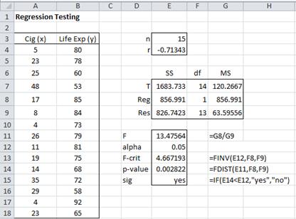
Example 1: Test whether the regression line in Example 1 of Method of Least Squares is a good fit for the data.
Figure 1 – Goodness of fit of regression line for data in Example 1
We note that SST = DEVSQ(B4:B18) = 1683.7 and r = CORREL(A4:A18, B4:B18) = -0.713, and so by Property 3 of Regression Analysis, SSReg = r2·SST = (1683.7)(0.713)2 = 857.0. By Property 1 of Regression Analysis, SSRes = SST – SSReg = 1683.7 – 857.0 = 826.7. From these values, it is easy to calculate MSReg and MSRes.
We now calculate the test statistic F = MSReg/MSRes = 857.0/63.6 = 13.5. Since Fcrit = F.INV(α, dfReg, dfRes) = F.INV(.05, 1, 13) = 4.7 < 13.5 = F, we reject the null hypothesis, and so accept that the regression line is a good fit for the data (with 95% confidence). Alternatively, we note that p-value = F.DIST.RT(F, dfReg, dfRes) = F.DIST.RT(13.5, 1, 13) = 0.0028 < .05 = α, and so once again we reject the null hypothesis.
Observations
There are many ways of calculating SSReg, SSRes, and SST. E.g. using the worksheet in Figure 1 of Regression Analysis, we note that SSReg = DEVSQ(K5:K19) and SSRes = DEVSQ(L5:L19). These formulas are valid since the means of the y values and ȳ values are equal by Property 5(b) of Regression Analysis.
Also by Definition 2 of Regression Analysis, SSRes = (yi – ŷi)2 = SUMXMY2(J5:J19, K5:K19). Finally, SST = DEVSQ(J5:J19), but alternatively SST = var(y) ∙ dfT = VAR(J5:J19) * (COUNT(J5:J19)-1).
Reference
Howell, D. C. (2010) Statistical methods for psychology (7th ed.). Wadsworth, Cengage Learning.
https://labs.la.utexas.edu/gilden/files/2016/05/Statistics-Text.pdf

Hi Charles,
If this test gives a non-significant answer, i.e. it is impossible to reject the null hypothesis, but the test regarding the slope gives a significant different value from zero, what conclusion should than be made?
Greetings,
DD
Hello DD,
Can you send me an Excel spreadsheet where this has happened?
Charles
Charles, how can we get the linier line of the regression? Can we write it manually after estimating the parameters?
Fariq,
Perhaps you are referring to the trendline. To draw the trendline in Excel, see the following webpage
https://real-statistics.com/excel-environment/excel-charts/
You can click on the Trendline option in the menu shown on the right side of Figure 5.
Charles
Dear Charles,
Is this equivalent of asking excel to run a regression analysis using the “Data analysis” package?
Is there any statistical test we should do to test linearity?
Pedro,
1. This data is displayed when you run Excel’s Regression data analysis tool. This webpage describes how to interpret this part of the results.
2. Create a scatter plot and see whether the data roughly aligns with a straight line.
Charles
Hi Charles, are these methods valid for multiple regression as well?
Jonathan,
Yes, but see
https://real-statistics.com/multiple-regression/
Charles
Thank sir
Hi Charles,
How does one test the assumption of linearity of the phenomenon measured? Sorry for the basic question.
Syifa,
The easiest method to determine whether is linearity between y and x is to create a scatter plot and see whether the points are reasonably close to a straight line.
Charles
No need to count anything? I was told that one can correlate between straight line and the data and produce a number. Forgot the source 🙁
I was wondering if the software can be used for things like this. Like I can see straight line in the scatter but my teacher doesn’t see that they are close…
Syifa,
You can correlate between the data and the corresponding points on the straight line. This is the square root of the R-square statistic from the regression analysis.
Charles
how to calculate Dof for SSreg?
See https://real-statistics.com/regression/regression-analysis/
Charles
The cells that you are using for calculations in the final Observation section must have been changed. There are no columns J, K, or L in Figure 1.
John,
These formulas are references to the spreadsheet in Figure 1 of the Regression Analysis webpage: https://real-statistics.com/regression/regression-analysis/
I have now updated the referenced webpage to make this clearer.
Thanks for bringing this problem to my attention.
Charles