Basic Concepts
It is often useful to create a model using simulation. Usually, this takes the form of generating a series of random observations (often based on a specific statistical distribution) and then studying the resulting observations using techniques described throughout the rest of this website. This approach is commonly called Monte Carlo simulation.
Worksheet Functions
Excel Function: Excel provides the following functions for generating random numbers.
RAND() – generates a random number between 0 and 1; i.e. a random number x such that 0 ≤ x < 1.
RANDBETWEEN(a, b) – generates a random integer between a and b (inclusive)
Note that these functions are volatile, in the sense that every time there is a change to the worksheet their value is recalculated and a different random number is generated. If you don’t want this to happen, then enter RAND() on the formula bar and press the function key F9. This will replace the formula RAND() with the value generated. Alternatively, you can copy the random number (or a range of random numbers) using Ctrl-C and then paste them back into the same location using Home > Clipboard|Paste and then selecting the Paste Values option.
RANDBETWEEN only generates integer values. If you want a random number which could be any decimal number between a and b, then use the following formula instead:
= a + (b − a) * RAND()
Excel 365 Function: Excel 365 provides the following dynamic array function with spillover (see Dynamic Array Formulas).
RANDARRAY(nrows, ncols, a, b): fills an nrows × ncols range starting in the current cell with random numbers between a and b inclusive.
RANDARRAY(nrows, ncols, a, b, TRUE): fills an nrows × ncols range starting in the current cell with random integers between a and b inclusive.
If omitted nrows, ncols, and b default to 1, and a defaults to 0.
E.g. to generate 10 random numbers between 0 and 1 using Excel 365, you enter the formula =RANDARRAY(10) in cell A1 and press Enter.
If you are not using Excel 365, you can instead enter the formula =RAND() in cell A1, highlight range A1:A10, and press Ctrl-D.
More Worksheet Functions
Real Statistics Function: The Real Statistics Resource Pack provides the RANDOM function which generates a non-volatile random number.
RANDOM(a, b, FALSE, seed) = random number between a and b; i.e a non-volatile version of a + (b − a) * RAND()
RANDOM(a, b, TRUE, seed) = random integer between a and b, inclusive; i.e. a non-volatile version of RANDBETWEEN(a, b)
If a is omitted it defaults to 0, if b is omitted it defaults to 1 and if the third argument is omitted it defaults to FALSE.
If seed ≤ 0 or omitted then no seed is used, while if it is a positive value, then this value is used as a seed. A seed can be used to generate a repeatable sequence of pseudo-random values.
The Real Statistics Resource Pack also provides the following array function.
RANDX(nrows, seed, ncols): returns an nrows × ncols array of non-volatile random numbers between 0 and 1 where seed is as for RANDOM; the default for ncols is 1.
Data Analysis Tool
Excel Data Analysis Tool: In addition to the RAND and RANDBETWEEN functions, Excel provides the Random Number Generation data analysis tool which generates random numbers in the form of a table that adheres to one of several distributions. You can specify the following values with this tool:
Number of Variables = number of samples. This is the number of columns in the output table generated by Excel.
Number of Random Numbers = the size of each sample. This is the number of rows in the output table generated by Excel.
Distribution desired: specifies one of the following distributions:
- Uniform, specify α (lower bound) and β (upper bound)
- Normal, specify µ (mean) and σ (standard deviation)
- Bernoulli, specify p (probability of success); like the binomial distribution with n = 1
- Binomial, specify p (probability of success) and n (number of trials)
- Poisson, specify λ (mean)
- Patterned – specify a lower and upper bound, a step, repetition rate for values, and repetition rate for the sequence
- Discrete – specify a value and the associated probability range. The range must contain two columns: the left column contains values and the right column contains probabilities associated with the value in that row. The sum of the probabilities must be equal to 1.
Random Seed = an optional value used to generate the first random number. You can reuse this value later to ensure that the same random numbers are produced. If this field is left blank, then a new random number will be generated each time.
Examples
Example 1: Simulate the Central Limit Theorem by generating 100 samples of size 50 from a population with a uniform distribution in the interval [50, 150]. Thus each data element in each sample is a randomly selected, equally likely value between 50 and 150.
Select Data > Analysis|Data Analysis and choose the Random Number Generation data analysis tool. Fill in the dialog box that appears as shown in Figure 1.
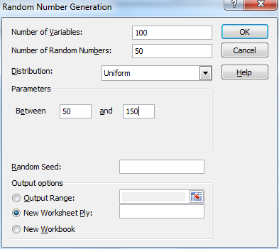
Figure 1 – Random Number Generator Dialog Box
The output is an Excel array with 50 rows and 100 columns. We next calculate the mean of each column using the AVERAGE function. The result is a row with 100 entries containing the means of each of the 100 samples. This is shown in Figure 2 (reformatted as a 10 × 10 array to fit on the screen better).
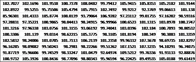
Figure 2 – Means of the 100 random samples
Using Excel’s Histogram data analysis tool we now create a histogram of the 100 sample means, as shown on the right side of Figure 3.

Figure 3 – Testing the Central Limit Theorem
Using the AVERAGE and STDEV.S functions, we calculate the mean and standard deviation of the 100 sample means from Figure 2. The mean of the sample means is 100.0566 (cell B7 of Figure 9.8.3) and the standard deviation is 4.318735 (cell B8). As you can see, the histogram is a somewhat imperfectly bell-shaped curve of a normal distribution.
Since the sample was taken from a uniform distribution in the range [50, 150], as can be seen from Uniform Distribution, the population mean is 

Based on the Central Limit Theorem, we expect that the mean of the sample means will be the population mean, which seems to be the case since 100.0566 is quite close to 100. We also expect that the standard deviation of the sample means to be
![]()
(cell B16) which is reasonably close to the observed value of 4.318735.
Random sample from a distribution
We can also manually generate a random sample that follows any of the distributions supported by Excel (or the Real Statistics Resource Pack) without using the data analysis tool. E.g. to generate a 25-element sample that follows a normal distribution with a mean of 60 and a standard deviation of 20, we simply use the formula =NORM.INV(RAND(),60,20) 25 times.
In column C (i.e. the column of x values) in Figure 4, we have done just that. E.g. cell C4 contains the formula
=NORM.INV(B4,$G$3,$G$4)
where cell B4 (and all the other cells in column B) contains the formula =RAND(). Column D contains the probability density values (i.e. labeled the y values) for each x value. E.g. cell D4 contains the formula
=NORM.DIST(C4,$G$3,$G$4,FALSE)
Finally, we create a scatter plot of the x values vs. the y values by highlighting the range C4:D28 and selecting Insert > Charts|Scatter as described in Excel Charts. The scatter plot shown in Figure 4 has the characteristic bell curve shape of the normal distribution.

Figure 4 – Creating a sample from a normal distribution
Drawing a random sample from a distribution
Similarly, we can generate random samples for any of the distributions supported by Excel (or the Real Statistics Resource Pack). E.g. to generate one element from the Poisson distribution with a mean equal to 7, we use the formula =POISSON_INV(RAND(),7) where POISSON_INV is the Real Statistics function described in Poisson Distribution.
We can also use the Real Statistics functions RANDOM or RANDX in place of RAND. This is especially useful if you desire a non-volatile random number or when you want to use a seed.
In Excel 365 environments, RANDX can be used as a dynamic array function. E.g. to obtain an estimate of the mean of the beta distribution with α = 4 and β = 6, you can perform a Monte Carlo simulation of size 10,000 via the worksheet formula =AVERAGE(BETA.INV(RANDX(10000),4,6)) to obtain a result such as 3.99901, which is close to the theoretical value of α/( α+β) = 4/(4+6) = .4. You can also use a seed such as in the formula = AVERAGE(BETA.INV(RANDX(10000,123),4,6)) to obtain .39985.
See Simulating a Distribution regarding the simulation of an unknown distribution.
Weighted random numbers
When using the Excel random number formula =RANDBETWEEN(1, 4), the probability that any one of the values 1, 2, 3, or 4 occurs is 25%. We now describe a way of varying the probability that any specific value occurs.
Real Statistics Function: The Real Statistics Resource Pack provides the following function.
WRAND(R1) = a random integer between 1 and n where R1 is an n × 1 column range of weights.
Example 2: Generate 20 random numbers from the set {1, 2, 3, 4} using the weights in range H4:H7 of Figure 5.
Thus, the probability of generating a 1 is 50/(50+10+20+20) = 50%, the probability of generating a 2 is 10/(50+10+20+20) = 10%, etc.
The result is shown in column J of Figure 5.
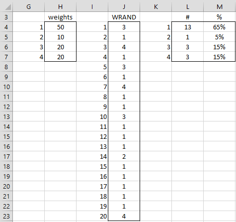
Figure 5 – Weighted random number generation
Here, each cell in range J4:J23 contains the formula =WRAND($H$4:$H$7). Range L3:M7 contains a tabulation of the number of times each of the values 1, 2, 3, and 4 occurs in the range J4:J23. E.g. cell L4 contains the formula =COUNTIF(J$4:J$23,K4). We observe that the frequency percentages in the range M4:M7 are similar (but not identical) to the probabilities that result from the weights.
Examples Workbook
Click here to download the Excel workbook with the examples described on this webpage.
Reference
Excel Easy (2021) Random numbers
https://www.excel-easy.com/examples/random-numbers.html
Hi Sir I need Solution for this question kindly help
Generate the hundred random numbers by using arena scheme then check these
numbers are uniformly distributed and have any correlation between these
numbers. You will consider seed square of your roll number.
𝒃
B. By using above generated random numbers to compute the ∫ 𝒆𝒙𝒑(
−𝒙
⁄ )𝒅𝒙 by
𝒂 𝟐
using the Monte Carlos simulation. Where you will consider the value of a is second
digit and b is first digit of your roll number.
1. Excel can generate random numbers, but I don’t know whether or not it uses the Arena scheme.
2. The Real Statistics RANDOM function enables you to use a seed.
3. I am in the process of adding new Bayesian statistics capabilities to the website and software. This will better support the type of Monte Carlo simulation that you have requested.
Charles
Hello,
I am using the following formula: =LOOKUP(RAND(),$D$4:$D$10,$B$4:$B$10). Row D represents number of times an event is happening and row B is the interval.
when I extend this formula to generate a simulation of 30 columns, it gives the same values instead of random values. Could you please tell me where did I make a mistake?
Hello,
I don’t use LOOKUP, but according to the following webpage
https://support.microsoft.com/en-us/office/lookup-function-446d94af-663b-451d-8251-369d5e3864cb
=LOOKUP(5,,$D$4:$D$10,$B$4:$B$10) should return the interval in column B that corresponds to the case where the number of times an event happens is 5 (as specified in column D). The problem is that when none of the values in column D is 5, the function uses the closest value. Now, instead of 5, you specified the value RAND(), which is a value between 0 and 1. If all the values in column D are bigger than 1, then the match will always be with the smallest value in column D since this is the closest to RAND() no matter what value RAND() takes (since it is always less than 1).
Perhaps you should use =RANDBETWEEN(a, b) instead of RAND() where all the values in column D are between a and b.
Charles
Hello im really new to this modeling and i have a question which is the same as your example. can i know like how to get a table and i cant find the option for the data analysis the generate random number thing please help
Sorry, but I don-t understand your comment.
Charles
File
Options
Add ins – go
Select “AnalysisToolpaK” from the list of avail Add-ins
OK
Charles,
You have provided very useful help with your post.
Thank you very much for taking time to do so.
The drilling productivity rate is the average depth reached in each type and different depth of soil per hour. (Pr=depth/duration)
We have the total duration of 1000 drilling piles.
Is there any method to measure the productivity?
Georges,
If I understand correctly you are looking for the productivity (depth per hour) for each of 4 soil types (A, B, C, D). If the productivity also varies by depth underground and say there are 5 different depths (1-10, 11-20, 21-30, 31-40, 41-50), then you have 4 x 5 = 20 different productivity values. One approach for calculating these 20 values is to use Excel’s Solver. You would assign arbitrary values to the 20 variables and then calculate the depth achieved for each of the 1000 drilling piles in your sample. You would then calculate the error between the theoretical depth based on the 20 productivity values and the depth actually achieved. You then need to calculate an overall error value (sum of squares or sum of absolute value or some other total error). You then use Solver to find the values of the 20 variables that minimizes the total error.
Charles
Hi Charles,
I have 1000 bored piles with the following data:
– pile depth
– soil type per depth (0-40,40-50,50-60 for each type of soil and I have 4 types)
– total drilling duration
How can I calculate the productivity for each depth with respect to soil type?
Your support is much appreciated.
Thank you
How do you measure productivity?
Charles
Hi there, please help with the following assignment! This would really be helpful.
Question 1
a) Place a formula in cell A1 that generates a random outcome from a normal distribution with mean = 10 and standard deviation = 2.
b) Place a formula in cell A2 that generates a random outcome from a uniform distribution with minimum = 0 and maximum = 5.
c) Place a formula in cell A3 that generates a random outcome from a right-skewed gamma distribution with shape parameter = 3 and scale parameter = 5 that covers the range [100, 250].
d) Place a formula in cell A4 that computes the coefficient of skewness for the gamma distribution of part c.
e) Place a formula in cell A5 that generates a random outcome from the left-skewed gamma corresponding to the right-skewed gamma of part c.
Question 2
Employees of Rider University are permitted to contribute a portion of their earnings to a flexible spending account from which they can pay medical expenses not covered by the University’s health insurance program. Contributions to an employee’s “flex” account are not subject to income taxes. The downside of “flex” accounts is that the employee forfeits any amount contributed to the account that is not spent during the year.
Suppose Joe Smith makes $60,000 per year and pays 33% in taxes. Joe estimates that in the coming year his family’s normal medical expenses not covered by the health insurance plan can be modeled with the following distribution
Amount $500 $1,500 $3,000 $4,000 $5,000
Probability 0.10 0.40 0.20 0.20 0.10
Joe also believes there is a 5% chance that an abnormal medical event could occur which might add $10,000 to the normal expenses paid from their “flex” account.
If uncovered medical expenses exceed the “flex” account contribution, Joe will have to cover these expenses with the after-tax money he brings home. Joe is considering contributing one of the following amounts to his “flex” account for the coming year: $1,000, $2,000, $3,000, $4,000. Use simulation to determine the amount of money Joe should contribute if he wants to maximize his disposable income (after taxes and all medical expenses are paid).
Clearly identify your recommended “flex” contribution, and write a brief paragraph in a text box justifying your recommendation.
Olivia,
I have a policy of not doing assignments. As a result, I will provide two hints:
1. See the following webpage regarding the gamma distribution:
Gamma Distribution
2. To generate a random value in Excel from a gamma distribution with parameters alpha and beta, you can use the formula =GAMMA.INV(RAND(),alpha, beta). The approach is similar for other distributions.
Charles
Dear Charles
I am constructing a non-inferiority trial with three intervention arms A, B, and C (placebo) related to a specific duration measured in minutes.
The hypothesis is that A>C, B>C, and non-inferiority between A and B. The non-inferiority margin is set to 25%, alfa 5%, beta 20%.
A has a mean (SD) of 800 (114), B 728 (114), C 570 (114).
How do I simulate the sample size with the above assumptions, means, and SDs? From a previous study utilising a similar design, data was found to be log-normal distributed. Is it even possible to use the random function for these data?
For the LogNormal distribution where you know the mu and sigma value, you can generate any number of random values using the formula =LOGNORM.INV(RAND(),mu,sigma). You can estimate the mu and sigma values from the mean and standard deviation as described at
https://www.real-statistics.com/distribution-fitting/method-of-moments/method-of-moments-lognormal-distribution/
Charles
Hi Charles,
Thanks for the content in your website. It is really useful!
I’m simulating some interest taxes that vary according to the number of months the customer paid for a product. There are 3 intervals with which I’m working: 1 month, 2 to 6 months and 7 to 12 months. For example: for the first interval, the tax is 4%; for the second, it’s 5%; for the third, 6%.
What I’m trying to answer is: is there any other combination that will maximize the company’s profit? I guess the answer is obvious (“yes, there is”), but I am trying to prove it quantitatively.
To start some simulations, I established some intervals in which each tax could vary. For example: 4% to 4,5% (1st), 4,5% to 5% (2nd) and 5% to 5,5% (3rd). After that, I used the formula you suggested: = a + (b-a)*RAND()
I repeated the formula 10,000 times for each interval and got some variations in the company’s profit. Finally, I plotted a histogram, with the variation in the profit (x axis) and the frequency they happened (y axis).
The point is: how can I use this histogram to answer my question? Is there a statistical basis to argue in which combinations the profit is more probable?
What I did was verifying which intervals of profit growth (in %) are “taller” in the histogram. Is that appropriate?
Thanks for your time and help.
Rafael,
A typical way to determine how to maximize a function is to use Excel’s Solver capability.
This is described on the Real Statistics website and many examples of how to do this are given.
Charles
Hi Charles,
First of all i want to thank you for this article and to thank you for your help.
I work actually on a simulation model where i need as input data the number of customers per hour of day. To this aim, i generated the distribution of customers inter arrival per hour. For example:
7AM:1 + 170 * BETA(0.52, 3.62)
8AM:LOGN(8.54, 10.2)
9AM:-0.001 + GAMM(3.61, 1.52)
10AM:LOGN(4.82, 3.98)
11AM:-0.001 + LOGN(5.5, 5.88)
Could you please help me to generate the number of customers please?
Thank you in advance
I don’t understand where you got the formulas for each time period.
If you are doing a simulation, you would usually use a formula such as =NORM.S.INV(RAND())
Generally, you would use exponential distribution for inter-arrival rates in queueing models. See
https://real-statistics.com/other-key-distributions/exponential-distribution/
Charles
Thank you for your Answer.
However, this formulas (Inter arrival distribustion per hour) are obtained from Arena Input Analyzer.
Based on the information that you have provided, I don’t know how to get the result that you are looking for.
Charles
Hi Charles,
Quick question: what algorithm do you use in the RANDOM() function to output given the seed? I tried to reproduce the function using the Lehmer random number generator and failed.
Thanks much
I used the one that Excel VBA uses.
Charles
Hi Charles
For the RANDOM function, is there a way to generate a series of random numbers of size n using only one SEED number.
Thank you
Andrew
Andrew,
It depends on what you mean by “using one seed number”. Let’s assume that a = 0, b = 1, n = 20 and seed = .512. One approach is to place the formula =RANDOM(0,1,,.512) into cell A1. I then place the formula =RANDOM(0,1,,A1) into cell A2. Next, I highlight the range A2:A20 and press Ctrl-D. This will give me 20 random values using one initial seed.
Charles
I have the same exact question (for a repeatable monte carlo simulation). Thank you Charles!
Thank you for this article.
How would you approach generating, say, 5 series of random numbers, each of which is correlated to the other four (based on a correlation analysis of past values of the 5 series)? I have seen some discussions online about using Rho in a two-variable setup; can you advise on a generalized approach for n variables?
Thanks!!
Hello Bill,
Let’s first look at the case with two series.
I can use the RAND function to generate say 10 random numbers between 0 and 1. This is the first series.
Now, I believe that you want to generate 10 numbers randomly so that the correlation with the first series is one (?!) Is this correct? Since the correlation is one, this means that there is a constant c such that the values in the second series are all c times the corresponding values in the first series. Since the first series was random, the second series should be random as well, but there is nothing random about the pair of series.
In any case, you can create as many of these series as you like by randomly selecting different values for the constant c.
Most likely, this is not what you intended by your question. Please clarify.
Charles
Thanks for your prompt reply!
What I meant is:
– E.g. 5 series of 100 elements each, randomly between 0 and 1
– each series of random numbers will display a degree of correlation to the others, e.g. per this correlation matrix (numbers made up for illustration, may not be consistent; but would be based on observed past behavior of the 5 series):
X1 X2 X3 X4 X5
X1 1
X2 0.3 1
X3 0.25 0.35 1
X4 -.5 0.2 -.6 1
X5 .5 .5 .4 .3 1
So procedurally, I’d like to
-Generate a series for X1;
-Then for X2, displaying a 0.3 correlation with X1
-Then for X3, displaying a 0.25 correlation with X1 and a 0.35 correlation with X2
etc.
-Bill
Hi Bill,
This is a very interesting question.
One way to address this sort of problem is first create k random vectors from a multinormal distribution with a specific mean vector and correlation matrix. This is described at
https://real-statistics.com/multivariate-statistics/multivariate-normal-distribution/random-multivariate-normal-vectors/
For each correlation r among the uniform distributions, the corresponding correlation for the multinormal distribution is 2*sin(r*pi/6) as described at
https://stats.stackexchange.com/questions/66610/generate-pairs-of-random-numbers-uniformly-distributed-and-correlated
Finally you need to transform the normally distributed data to uniformly distributed data by using the NORM.S.DIST function.
For two uniform distributions with correlation .3 you can follow the following steps:
1. Set cell A1 to .3 and cell B1 to =2*SIN(A1*Pi()/6). Thus cell B1 will contain the value .312869
2. Place the array formula =TRANSPOSE(BNORMRAND(0,0,1,1,B$1)) in range A3:B3, highlight the range A3:B102 and press Ctrl-D. This range now contains the appropriate data from a binormal normal distribution.
3. Place the formula =NORM.S.DIST(A3,TRUE) in cell D3, highlight range D3:E102 and press Ctrl-R and Ctrl-D. Range D3:E102 should now have the desired result.
The approach is similar for 5 samples instead of 2. This time you need to specify the 5 x 5 correlation matrix you want. You then need to transform this matrix to contain the correlations for the normal distribution (as above). Now you use the MNORMRAND function instead of BNORMRAND.
Charles
Many thanks to you, Charles.
The MNORMRAND function is wonderful for this purpose! I first used the COV() function to describe the interrelationships of the variables in the historical data, and used that as an input for MNORMRAND. It is working exactly as needed.
Thanks not only for your help, but for this whole Real-Statistics resource, which is very rich and useful.
Bill
Hi Charles, Could you please tell the step-by-step process for obtaining a histogram of the sample mean of 100 samples?
Hi Charles,
How can I simulate a sample of 100 observations using RANDBETWEEN(0,11) in Microsoft Excel but with a chosen mean of 3? (Poisson distribution). The numbers I generated using RANDBETWEEN(0,11) couldn’t give me the mean I wanted and it changes each time I edit something in the sheet. What should I do? Is there any other formula syntax in MS Excel for this function?
Hello Nicco,
You can use the Real Statistics function POISSON_INV which generates the inverse of the Poisson distribution. The specific formula to use is
=POISSON_INV(RAND(),3). You repeat this formula 100 times (e.g. place this formula in cell A1, highlight the range A1:A100 and press Ctrl-D).
The results will change each time you edit something on the sheet. To avoid this, you can use the formula =POISSON_INV(RANDOM(),3) instead.
Charles
Good day sir, please how can I use Excel simulation to generate response by Customers on service quality at a Train Station to be denoted as true=0 which means no complaint about the service quality and false=1 where any complaint exists and the service quality is dis-satisfactory. The responses will be for a number of customers between 1 and 820. Thank you, sir.
Good day sir, please how can I generate random numbers between 1 and 820 using excel for a response on service quality, where true=0 means no complaint about the quality and false=1 where any complaint exists and the service quality is dissatisfactory. Thanks sir.
David,
If the number must be an integer then use =RANDBETWEEN(1,820). If any decimal number will do, then use RAND()*819+1.
Charles
Hi Charles,
I wanted to make a random dice roll for 10 rows, and then each column will calculate whether the previous cell was bigger than 1, and if it was, it would repeat the first column’s dice roll. I have created this, but now I want to know if there is a way to count how many times a random number is generated within a cell and count it up every time it is recalculated, i.e. If cell A1 contains 2, and cell B1 contains 5, then it would add a 1 to the count in column 2. However if the next dice roll makes A1 contain a 1 instead, then cell B1 would contain nothing, yet the count would still equal 1 from the last time.
Thank you!
Lewis,
I don’t completely understand the scenario. Can you give me an example of a typical result?
Charles
Hi Charles,
Thank you for the article.
I want to create a random sample for “age”. I only know the mean (e.g: 35) and standard deviation (e.g:18). If I create a random sample using NORMINV(RAND(), 35, 18), I will get negative values. Could you please help me around this situation.
Thanks
Himani,
This shows that the real distribution is not completely normal. The only thing I can think of is to eliminate all the negative values. Since NORMDIST(0,35,18,TRUE) = 2.6%, this means that you only eliminate about 2.6% of the values.
Charles
Thank you Charles,
Would having the range (1 – 108) help ?
Himani,
Sorry, but I don’t understand what 1-108 refers to. What does the range 1-108 represent?
Charles