I am pleased to announce Release 7.6 of the Real Statistics Resource Pack. The new release is now available for free download at Download Resource Pack for Excel 2010, 2013, 2016, 2019 and 365 in both Windows and Mac environments.
The Regression 1 and Multivariate examples workbooks will shortly be updated for compatibility with the new release. Over the course of the next few days, the website will also be updated for compatibility with the new release.
If you are getting value from the Real Statistics website or software, I would appreciate your donation to help offset the costs of the website by going to Please Donate.
The following is an overview of the new features in Release 7.6:
Bivariate Normal Distribution
An improved algorithm has now been used to calculate the cdf for the BNORMSDIST and BNORMDIST functions based on
Genz, A. (2009) TVPack, Biivariate normal distribution
http://www.math.wsu.edu/faculty/genz/software/fort77/tvpack.f
In addition, the following two new functions have been added that enable you to specify a rectangular range of values:
BNORMSRECT(x1, x2, y1, y2, r, cum) = P(x1 < x < x2 and y1 < y < y2) for the standard bivariate normal distribution with correlation coefficient r.
BNORMRECT(x1, x2, y1, y2, mx, my, sx, sy, r, cum) = P(x1 < x < x2 and y1 < y < y2) for the bivariate normal distribution with means mx and my, standard deviations sx and sy and correlation coefficient r.
Minimum Spanning Tree
Adds the ability to create a minimum spanning tree for a network of nodes and undirected, weighted edges based on the Kruskal and Prim algorithms. This is achieved via the new array functions MSTKruskal and MSTPrim.
In addition, the following new array function has been added to find the minimum spanning tree between points in r-dimensional space.
MSTVectors(R1, brief, p, Rw): returns the minimum spanning tree for nodes in R1
R1 an n × r array consisting of n nodes, each of which is an r-tuple of real values. Each node is represented by its row number, 1 to n, in R1.
When brief = TRUE, the output consists of an n-1 × 2 array that represents the spanning tree, each row of which consists of a pair of node numbers showing which nodes are connected in the minimum spanning tree (these are the edges).
When brief = FALSE (default) the output contains an extra column that specifies the distance between the corresponding two nodes.
The minimum spanning tree minimizes the sum of the edge weights in the tree. Here, the weight of an edge is the distance between the two nodes that are connected by the edge. Since the nodes correspond to r-tuples in space, we can use the Euclidean distance when p = 2 (default). Alternatively, we can use the Minkowski distance, corresponding to the Lp norm, for other values of p. E.g. we can find the Manhattan minimum spanning tree when p = 1, in which case the Manhattan distance is used.
In addition to the unweighted Lp norm described above, we can use a weighted Lp norm as the distance function. In this case, the optional r × 1 array Rw is used to specify the weights for each of the r dimensions. If Rw is omitted then the unweighted Lp norm is used.
Friedman-Rafsky Test
The Friedman-Rafsky test is a multidimensional version of the Wald-Wolfowitz runs test and can be used to test whether two multivariate samples come from the same distribution.
FR_Test(R1, R2, lab, p, Rw): returns a column array with the values: size of sample 1, size of sample 2, test mean, test standard deviation, # of runs, z-stat, p-value.
Here, R1 and R2 contain the data in the two samples, each consisting of r-tuples where r = the number of columns in R1, which is the same as the number of columns in R2. If lab = TRUE (default FALSE), then an extra column of labels is appended to the output.
This test uses a minimum spanning tree whose nodes are the r-tuples from the combined samples and whose edge weights are the distances between the nodes based on the distance metric defined by the p and Rw values as described above for the MSTVectors function. p defaults to 2 (Euclidean distance) and Rw is omitted if no weights are used.
The # of runs is equal to the number of edges in the minimum spanning tree that connect two nodes from different samples.
Charting of networks of nodes and edges
A new Network Diagram data analysis tool has been added that displays networks of nodes and edges, as described above, using Excel’s charting capability.
The inputs to this data analysis tool are the Nodes range and Edge range, each of which contains two columns. The output from the analysis tool is a chart that displays the nodes in the Nodes range as points in two-dimensional space connected by lines as specified in the Edge range.
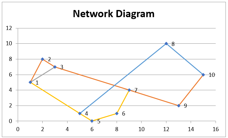
The Nodes range consists of an n × 2 cell range which specifies n two-dimensional points. The row numbers in this range are used to specify the nodes. Each row in the Edge Range consists of a pair of node numbers that are connected by an edge.
Lp Regression
Added functionality that supports Lp Regression based on using the Lp norm, introduced in Release 7.4, when calculating the error value. When p = 1 this is identical to LAD regression.
The following new functions have been added: LpRegCoeff, LpRegWeights, LpRegCoeffSE. These functions provide similar capabilities to LADRegCoeff, LADRegWeights, LADRegCoeffSE. In fact, when p = 1 they produce the same output. These functions also take the same arguments as the corresponding LAD functions except that the value of p is inserted as the fourth argument.
Eigenvalues and eigenvectors
Improved the eigVECTSym function so that it automatically generates mutually orthogonal eigenvectors. If there are any imaginary eigenvalues then this function now generates an error value.
Added the eigVECTReal function. This function is identical to the previous version of the eigVECTSym function. Also added the eigVALReal function which is equivalent to the eigVALSym function.
Also added the following array function that supports repeated eigenvalues.
eigMultVECT(R1, lambda, prec): outputs an array whose columns are mutually orthogonal eigenvectors corresponding to the eigenvalue lambda for the square matrix R1; prec is a small positive number (default .0001) where values ≤ prec are treated as if they were zero.
Bug Fixes
- Fixed a bug in the HC1 version of robust errors in the RRegCoeff and RR0Coeff functions.
- Updated Ridge regression capabilities when there is only one independent variable. This applies to the Ridge Regression data analysis tool as well as the RidgeRegCoeff, RidgeMSE and RidgeLambda functions.