Basic Concepts
One problem that we face in analyzing data is the presence of outliers. Outliers are data elements that are much bigger or much smaller than the other data elements.
For example, the mean of the sample {2, 3, 4, 5, 6} is 4, while the mean of {2, 3, 4, 5, 60} is 14.4. The appearance of the 60 completely distorts the mean in the second sample. Some statistics, such as the median, are more resistant to such outliers. In fact, the median for both samples is 4.
For this example, it is obvious that 60 is a potential outlier. In Identifying Outliers and Missing Data we show how to identify potential outliers using a data analysis tool provided in the Real Statistics Resource Pack.
You can use a Box Plot as described in Box Plots with Outliers to identify potential outliers. Alternatively, you can use the approach described in Identifying Outliers and Missing Data or Grubbs Test.
Trimmed Mean
One approach for dealing with outliers is to throw away data that are either too big or too small. This is usually not recommended, although trimming the data is often used. Excel provides the following function for doing this.
Excel Function: Excel provides the following function to calculate a trimmed mean.
TRIMMEAN(R1, p) – calculates the mean of the data in R1 after first throwing away 100p% of the data, half from the top and half from the bottom. If R1 contains n data elements and k = the largest whole number ≤ np/2, then the k largest elements and the k smallest elements are removed before calculating the mean.
For example, suppose R1 = {5, 4, 3, 20, 1, 4, 6, 4, 5, 6, 7, 1, 3, 7, 2}. Then TRIMMEAN(R, 0.2) works as follows. Since R1 has 15 elements, k = INT(15 * .2 / 2) = 1. Thus the largest element (20) and the smallest element (1) are removed from R1 to get R2 = {5, 4, 3, 4, 6, 4, 5, 6, 7, 1, 3, 7, 2}. TRIMMEAN now returns the mean of this range, namely 4.385 instead of the mean of R1 which is 5.2.
Winsorized Samples
A related approach to trimming is to use Winsorized samples, in which the trimmed values are replaced by the remaining highest and lowest values. Consider the following sample with 20 elements:
4, 6, 10, 14, 16, 19, 22, 23, 25, 27, 27, 31, 37, 38, 40, 44, 45, 48, 50, 80
A 20% trimmed sample would simply remove the two lowest and two highest elements (i.e. 4, 6, 50, 80). A 20% Winsorized sample replaces the two lowest elements by the third lowest element and the two highest by the third highest element, resulting in the following data set:
10, 10, 10, 14, 16, 19, 22, 23, 25, 27, 27, 31, 37, 38, 40, 44, 45, 48, 48, 48
The Winsorized mean of the original sample is the mean of the Winsorized sample, which in this case is 29.1 (instead of 30.3 for the original sample).
Observation: Since four data elements have been replaced, the degrees of freedom of any statistical test needs to be reduced by 4.
Worksheet Functions
Real Statistics Functions: The Real Statistics Resource Pack supplies the following functions:
TRIMDATA(R1, p): array function which returns a column array equivalent to R1 after removing the lowest and highest 100p/2 % of the data values.
WINSORIZE(R1, p): array function which returns a column array which is the Winsorized version of R1, replacing the lowest and highest 100p/2 % of the data values.
WINMEAN(R1, p) = Winsorized mean of the data in R1 replacing the lowest and highest 100p/2 % of the data values.
Example 1: Find the 30% trimmed and Winsorized data for the sample in range A4:A23 of Figure 1. Also, find the corresponding trimmed and Winsorized means.
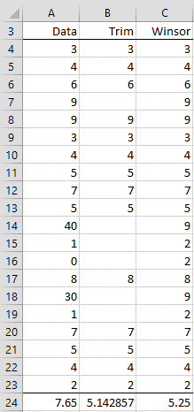
Figure 1 – Trimmed and Winsorized Data
Range B4:B23 contains the trimmed data in range A4:A23 using the formula
=TRIMDATA(A4:A23,.3)
The trimmed mean (cell B24) can be calculated using either of the formulas
=TRIMMEAN(A4:A23,.3) or =AVERAGE(B4:B23)
Range C4:C23 contains the Winsorized data in range A4:A23 using the formula
=WINSORIZE(A4:A23,.3)
The Winsorized mean (cell C24) can be calculated using either of the formulas
=WINMEAN(A4:A23,.3) or =AVERAGE(C4:C23)
Worksheet Function Extensions
Real Statistics Functions: Each of the functions described above can optionally take a third argument q. In this case, the action on the lowest data values is governed by p and the action on the highest data values is governed by q.
TRIMDATA(R1, p, q): array function that returns a column range equivalent to R1 after removing the lowest 100p % of the data values and the highest 100q % of the data values.
WINSORIZE(R1, p, q): array function which returns a column range which is the Winsorized version of R1 replacing the lowest 100p % of the data values and the highest 100q % of the data values.
WINMEAN(R1, p, q) = AVERAGE(WINSORIZE(R1, p, q))
Note that TRIMDATA(R1,p,p) is equivalent to TRIMDATA(R1,2*p) and WINSORIZE(R1,p,p) is equivalent to WINSORIZE(R1,2*p).
In addition, there is a new Real Statistics function that extends the Excel function TRIMMEAN, defined as follows:
TRIM_MEAN(R1, p, q) = AVERAGE(TRIMDATA(R1, p, q))
Note that TRIM_MEAN(R1, p) = TRIMMEAN(R1, p)
Examples Workbook
Click here to download the Excel workbook with the examples described on this webpage.
References
Wikipedia (2012) Winsorizing
https://en.wikipedia.org/wiki/Winsorizing
Microsoft Support (2012) TRIMMEAN function
https://support.microsoft.com/en-us/office/trimmean-function-d90c9878-a119-4746-88fa-63d988f511d3
When using trimdata on my array it is just returning the first value in the array repeatedly. How do I fix this? Thanks
Cary,
TRIMDATA is an array function and so you can’t simply press the Enter key. It is not hard to use such functions, but you need to use the proper approach. This is described at
Array Formulas and Functions
Charles
Hello Charles,
Thank you so much for your perfect add-on. It helped me a great deal thus far.
You describe that the output of your TRIMDATA and the WINSORIZE function is a column range.
My predicament is that my dataset is structured in a matrix format (X being calendar week and Y is the year); thus I was wondering whether there is a possibility to get the output in the same format as the input range? I could transpose the dataset, but for the sake of visibility, currently the matrix format suits best.
Thank you very much in advance !
Best
Max
Hello Max,
You can change the shape of any output by using Real Statistics’ RESHAPE function.
To trim the data in range R1, you can highlight a range of the same shape as R1 (or any other shape for that matter) and use the array formula =RESHAPE(TRIMDATA(R1)).
Charles
Hi Charles,
amazing. Exactly what I had hoped for.
Thanks again !
Max
Hello Charles, one more question.
It seemed that the WINSORIZE function accepts two parameters p (lowest data values) and p1 (highest data values). Maybe I am missing something, but the array only seems to make a change in both tails, not the right tail only, if I keep p = 0 and p1=0.05.
I was trying to achieve something like this: {=RESHAPE(WINSORIZE(B4:BA9,0,0.05))}
I know that some of my data points under the right tail are outliers and I’d like to adjust only those.
Thanks
Max
Hello Max,
Yes, you are correct. The WINSORIZE function doesn’t handle the right tail properly. I will fix this in the next release, which is due out within one week.
Thank you very much for identifying this error.
Charles
I would like to winsorise at 1% and 99% of data. Can I check how I should do this and what resource pack will you recommend me to download. Thanks
Melody,
You can use the WINSORIZE function, although it is likely that your data set is so small that eliminating 1% of the data on each end doesn’t eliminate any data. If so, you need to increase this percentage.
Charles
Hi Charles! I officially owe you a beer! I had a question, but I’ve managed to figure it out. Your “Winsorizing” function has totally saved the day! I’m using it for a complicated art project – if it is at all successful I’ll make sure to credit your contribution! Keep up the good work!
B. Evans
Ben,
Glad I could help you out. I am look forward to that beer.
Charles
Hello Charles,
I have a question regarding the example for using the function WINSORIZE and TRIMDATA. I downloaded the function as a plug-in. And I also downloaded the example. But I have a problem. When I use these functions I only get the data in C4 or E4. I don’t get the data for the rest of the column. How do I get data for the entire column and not just for the first one?
Kind regards,
Patrick,
TRIMDATA and WINSORIZE are array functions, and so you can’t simply press Enter to get the complete output. Instead you need to highlight the range where the output goes and press Ctrl-Shft-Enter. See the following webpage for more details on how to handle array functions.
Array Formulas and Functions
Charles
Dear Charles,
I am trying trim my data set that is structured like this:
Object Observation Trimmed observations
A 10
A 12
A 24
…. ….
B 123
B 111
B 500
…. ….
C 1234
C 1100
C 5000
My objective here is to trim all observations belonging to Object A, followed by Object B, and so on. I can imagine doing them manually would be very time consuming, especially if there are many different objects.
Is there a way which I can code the cells on the column “Trimmed observations” such that I can trim the collective observations of each object separately from the entire observations of all objects combined? The scale of observations from A, B, and C are very different, and trimming their combined data would surely result from removal of data from A and C.
Hope you can help! Thank you so much.
Joe,
You could use the Real Statistics TRIMDATA function three times, one for each range.
Charles
Hello Charles,
I have two questions:
1. If using TRIMMEAN function, how to decide if we should take a cut off value as 20% or 30%?
2. If using TRIMMEAN, and for example it removes 2 lowest data points (0,1 for example) but I have one more data point as “1” so it will remove one “1” and will not remove the another “1” so is that nor wrong?
2. Which is the best method to remove outliers out of TRIMMEAN, IQR method and mean / std dev method (the one with +-2.5 cut off)?
Goyal,
1. There is no definitive answer here. You should enter a value that is big enough to eliminate any outlier; ideally you want the smallest such value.
2. That is correct. If you want both to be removed, then enter a higher cutoff value.
3. Again, there is no definitive answer.
Charles
Hi Charles ,
could you provide me with the excel sheet for the posted example as i tried to do it my self but i couldn’t
thanks
keshk
Keshk,
See the webpage Examples Workbooks.
Charles
Hi Charles
Thank you again for this excellent website, the resource pack and your availability concerning one of my problems you fixed recently regarding Kendall W.
I have a question regarding a set of data containing missing data at random and potential outliers that potentially impact the multiple regression i processed on the dataset, using only listless deletions that really shrieked the sample size.
To look for a better fitting multiple regression model, i’d like to apply the methods you describe regarding missing data and outliers.
But should I first perform identification (+/- removal and replacement) of outliers using winsorize (for exemple) and then multiple imputation using FCS for missing data?
or the opposite? (could it creates a bias in the multiple imputation?)
and by the way, once the multiple imputation process is done as you describe it in your website, how can i manage to finally replace the missing data by the new data generated through the MI to run a new series of analysis?
Thank you very much for your help.
Louis
Louis,
I don’t know for sure, but it probably depends on the nature of the outliers. If the outliers are errors in data collection or reporting, then you should probably remove them first, but if they represent real data, then you probably shouldn’t remove them at all. If you need to remove them to make the assumptions for some test to work, then you should report this fact when you state your results.
When you use MI, you repeat the regression analysis a large number of times with different values for the missing data. This enables you to complete your analysis, but there is no set of values imputed for the missing data elements.
Charles
hi charles
I am working on excel 2007
I want to find outliers in the data as a assignment but not gettng the function trimmean
can you tell me
Kajol,
TRIMMEAN is a standard Excel function which is available in Excel 2007.
Charles
Hi Charles,
installed everything succesfully, but once i run winsorize fuction, only bottom top 5% are adjusted, but top range remains untouched. do you know what might be the issue?
If you send me an Excel file with your data I will try to figure out what is going wrong. You can find my email address at Contact Us.
Charles
hi Charles
I’m trying to do a one way anova test. when I use my original data the k-s test and leven’s test are ok but the result of my anova test is not meaningful. when I replace my outliers (extreme values) or transformed them the result my anova test becomes meaningful but not the levene’s test which is a problem because Homogeneity of Variances is one of the conditions of one way anova test in the first place.
don’t really know what to do? thanks
Hi Sohail,
When you say “meaningful” do you mean “significant” or “not significant” or something else?
It sounds like you get different results based on whether or not you include some outliers. This is a plausible outcome and is a credible result from the tests. You should now focus on whether the “outliers” represent normal random outcomes (e.g. in say 500 observations, you expect some outliers) or some problem (in measurement or something else). If the outliers represent normal events, then I would use your first result. If not I would use both results, unless you can find some way to remove the causes of the outliers.
Charles
yes sorry by meaningful I meant significant
so if I replace my outliers I have to redo the Levene’s test and the k-s test with the new data set? cant’t I use the original data for the Levene’s test and the K-S test and replace the outliers only for the one way anova test?
Thank you for your help
Sohail,
It is not clear to me why you need to use the KS test at all.
In any case, if you change your data, then you need to check normality (presumably using Shapiro-Wilk) and homogeneity of variances (e.g. Levene’s test) for this data. You are probably ok provided the variances are not too unequal, but if they are then you mighyt want to consider using Welch’s ANOVA test instead of the usual ANOVA.
Charles
Good afternoon Charles,
I am learning a lot through this web course, but I am still having some issues that I hope you can easily address.
I have a data set of 25-50 data points. I want to run the grubbs outlier test on this data set and then have it report the numbers that are not outliers. The results of this will then be used to calculate the average.
For example: {1,2,3,4,5,10} is my data set, after finding the grubbs outlier {10} and removing that number from my calculations, the average is 3.
How might I achieve my desired results using an Excel spreadsheet. Thank you in advance for any advice you may provide.
Hello Phillip,
Please see the following webpage for information about how to conduct Grubb’s outlier test in Excel.
Grubb’s Outlier Test
Charles
Hi charles..
Thank you providing me some information about winsorize data.
I need your help with my data collection. I want to evaluate data by using logistic regression but my independent variables are continuous data. So it have outliers and spikes.
My questions is when I choose to winsorize my data, how to determine the value of p? are the value of p is same as each variables or refer to the outliers?
i give you example of my data.
[0.0789 0.0743 0.0698 0.0758 0.0870 0.0767 0.0720 0.0781 0.0752 0.0695 0.0832 0.0869 0.0828 0.0777 0.0814 0.0751 0.0592 0.0661 0.0696 0.0624 0.0574 0.0457 0.0559 0.0572 0.0607 0.968 0.899 0.969 0.839 0.804 0.078 0.069 0.080 0.081 0.083 0.102 0.091 0.108 0.102 0.102 0.092 0.092 0.083 0.085 0.091 0.088 0.084 0.091 0.088 0.098 0.066 0.071 0.074 0.074 0.090]
how i decide the value of p?
can u help me?
Sorry, but I don’t have any specific advice. Your goal is to remove outliers and reduce skewness.
Charles
Hi Charles,
Thanks for sharing your AddInst. I believe many people feel this is very useful for them. However, I got an issue relating winsorizing. I tried to winsorize my data with 1% (percentile 1% and 99%). I typed =WINSORIZE($C$2:$C$993,.01) using your AddIns and it was going well. However, after comparing the value produced by Excel (the value of 1% and 99% percentile) and the result of the AddIns I found them different. Could you help me what causing the difference?
Thanks in advance for your assistance.
Andri
Andri,
The WINSORIZE function is an array function, which outputs the values to retain after Winsorizing data. Excel has a WINMEAN function which outputs a single value which should be the mean of the values produced by the WINSORIZE function. Thus the result of AVERAGE(WINSORIZE($C$2:$C$993,.01)), after pressing Ctrl-Shift-Enter, should be the same as WINMEAN($C$2:$C$993,.01), after pressing Enter.
If you send me an Excel file with your data, I can check to see whether there is a problem.
Charles
Hello Charles,
I used your formula “{=winsorize(A$1:A$62780, 0.03)}”
When I drag it down, I have the same answer for every cells.
This might be due to the range of cells to hold the answer..
How can I properly select the range of cell to hold the results (and therefore, get the desired results)
Hope you understand my issue.
Thank you,
Valentine
Valentine,
Suppose you want to place the output in range C1:C62780. Since WINSORIZE is an array formula, you need to highlight the full range C1:C62780, enter the formula WINSORIZE(A$1:A$62780, 0.03) and press Ctrl-Shift-Enter.
The result will copy all the values from A1:A62780 replacing the low and high values by blanks.
Charles
Hey Charles
I followed your methods above using the winsorise method and only one number appear from the array
When I tried the crl shift enter the whole range appears as usual, with no blanks for the outliers. is the formula not working
I was unable to get your functions to work as expected. The macros installed just fine, but they don’t seem to give correct results. It would be very beneficial is you published an example .xlsx file that contains the example you gave in the article. That way I could look at your working example and figure out what I did wrong.
Doyle,
You can download an Excel file with all the examples on the website from the webpage Download Examples.
Charles
Ah, that helps. Discovered my first problem is that the equations are not compatible with Excel tables.
Even without tables I still cannot reproduce your functionality. The input range to the Winsorize() function shifts on each cell. (e.g. it’s A1:A10 on the first cell, A2:A11 on the second, etc.)
And if I fix it in place using the $A$1 notation then all cells have the same value.
Any thoughts?
Doyle,
The WINSORIZE function is an array function. If for example your data is in range A1:A10 and you want to display the result in range C1:C10, you need to highlight range C1:C10 and enter the formula =WINSORIZE(A1:A10,.4) (here I have set the p value to .4) and press Ctrl-Shft-Enter.
To get more information about how you use array formulas and functions in Excel, refer to the webpage
Array formulas and functions
Charles
Hello Charles:
I located your site (and the software you have, thank you) when attempting to calculate a Standard Deviation using trimmed data. Needless to say this was an exercise in futility with native Excel 2007 (later releases don’t help here either).
I have downloaded and installed you software and am encountering a problem using one of the functions TrimData. Before I describe the error I will first describe the data being used.
The data is stock data (about 7000 entries) which has been downloaded and loaded into a table. Various calculations are performed on a row by row basis and stored in various columns, one of which is a calculated percent. The data in this column is then placed (copied) in other columns (of which there are 10) based upon the price range that the stock falls into (<<$5, $5-$10, $10-$25,…) and are labeled in the table according to a category number that corresponds to the price range (Cat1, Cat2, Cat3, …). Given the above that would mean only 1 column in any 1 row would have data and the others would be blank.
It is each one of these columns that I would like get the Standard Deviation after the data has been trimmed. To trim the data I created 1 more column (to become 10 once I get it working) and added the TrimData function into the first cell of the newly created column with the intent to copying it to the remaining cells in that row.
I've tried various formats of the TrimData and get #Value error or a syntax error depending on the format used. Below are the various syntax used and the results:
1. =trimdata([Cat1],0,3) #Value! error
2. {=trimdata([Cat1],0,3)} #Value! error
3. =trimdata(Table36[Cat1],0,3) #Value! error
4. {=trimdata(Table36[Cat1],0,3)} #Value! error
5. =trimdata(T11:T17,0,3) #Value! error Data contain a blank in the columns
6. {=trimdata(T11:T17,0,3)} #Value! error "" ""
7. =trimdata(T13:T17,0,3) #Value! error Data did not contain a blank in the columns
8. {=trimdata(T13:T17,0,3)} #Value! error "" ""
I also tried several of the above using a ";" (as Timo had in his entry) and a ":" (which you used in your response to Timo).
I used an [Enter] and a [CTL+SHFT+Enter] for all of the various formulas.
I assume I am doing something wrong here but I can not see it.
My intent here is to use the results of the trimmed data as input to the STDEV or SDDEVP. Once this is working I will experiment with the other trimming techniques you have supplied in this software.
Can you please help?
Thank you for your assistance and for providing this software.
Frank,
If you send me an Excel spreadsheet with your data I will try to figure out what is going wrong. See Contact Us for email address.
Charles
Hi Charles,
I would like to winsorize my outliers (identified by outlier labelling rule), but I am unsure which number I should replace them with because of my experimental design. Two groups have been measured four times. Should I replace the outliers with 1) the highest/lowest value in the entire dataset 2) the highest/lowest value in the data from the group where the outlier was found or 3) the higest/lowest value in the data from the group and particular time point where the outlier was found.
Hope this makes sense.
Best regards,
Tanja
Tanja,
As usual, it really depends on how you will use the data subsequently, especially based on which tests you will run. E.g. if you are going to analyze the data by group, then probably choice 2 is the right one. I am not sure what choice 3 means.
Charles
Hi charles,
Can you tell me step by step how to WINSORIZED the data?
I’d already follow your step but still doesn’t work. My data’s range C2 : C499
Thankyou
I don’t know why you aren’t able to get the winsorize process to work. The steps are described on the referenced webpage. In any case, if you send me an Excel file with your data I will try to see why you aren’t able to winsorize your data.
Charles
Greeting Charles,
I have problem in locking the cells. I suppose the array of comparison should be same for all the cells?
{=TRIMDATA($F$2:$F$169;0,025)}
Gives same value to all the cells. Same with
{=WINSORIZE($F$2:$F$169;0,025)}
Should i use for cell locking € symbol? My country belongs to EuroZone.
Timo,
Even if your country uses the euro you should still use the dollar sign $ for absolute addressing.
Charles
Greetings Charles,
Heh heh yes, yes. In that case I think I am not sure am I using the trimdata formula correctly.
formula {=TRIMDATA($F$2:$F$169;0,03)} gives same number/result for each cell. I use the formula identically for each cell from 2 to 169.
Thing is that I am not sure how the array works in general..
If range is F2:F169 and I input the results of function into H2:H169 then for row 2 the formula should be for each cell anyway the same?
What I mean to ask is that is this trimming certain amount of percentage from population or from value?
I need to trim certain percentage from population outliners.
It would be great if you could add an video and clarify the usage of the formula in the video :). Anyway, I appreciate your time to answer and great that this package is free =)
Timo,
Suppose your input data is placed in the range F2:F169. This range consists of 168 cells. .03 times 169 = 5.04. Half of this value is 2.52. You need to round down to the nearest integer, namely 2. This means that in calculating {=TRIMDATA($F$2:$F$169;0,03)} the lowest two values in F2:F169 will be replaced by blanks and the highest two values in F2:F169 will be replaced by blanks.
If you highlight the range H2:H169 and enter the formula {=TRIMDATA($F$2:$F$169;0,03)} and then press Ctrl-Shft-Enter the values in range H2:H169 will be identical to the values in range F2:F169 except that the lowest two values will be replaced by blanks and the highest two values will be replaced by blanks.
Note also that =AVERAGE(H2:H169) will have the same value as =TRIMMEAN(F2:F169:0,03).
Please see the webpage Array Functions and Formulas for more information about how to use array formulas in general.
Charles
Hi Charles,
I have the same problem with the WINSORIZE command as Mohammad. Unfortunately, it doesn’t work despite Ctrl-Shift-Enter. Are there any other things I overlooked?
Thank you very much for your help!
Maria
Maria,
I just checked and it certainly works on my computer. When you try to use the WINSORIZE function what sort of result do you get? An error value? a single number?
Make sure that you enter the formula in the form WINSORIZE(R1, p) where R1 is a range and p is a number between 0 and .5. Also make sure that you enter the formula into a range which contains a sufficient number of cells to hold the answer (if in doubt highlight a range of similar size to R1). Also don’t enter the formula into any cells that overlap with range R1.
Charles
Charles,
I have the same problem with the WINSORIZE command as Mohammed and Maria. Unfortunately, the Ctrl-Shift-Enter also doesn’t work. Can you help me?
Kind Regards
Heike
Heike,
Ctrl-Shift-Enter is how Excel recognizes an array formula. This doesn’t have anything to do with the Real Statistics Resource Pack, and so if this doesn’t work then your Excel software is flawed. Since I doubt this is true, please provide me with some more details so that I can better determine the problem. If you like you can send me an Excel spreadsheet with your data and what you have done and I can try to figure out what has gone wrong.
Charles
Charles
Thank you for your response.
=WINSORIZE($BS$2:$BS$6149;0,02), this is what I use. It is a quite big excel file. In every cell I get the same as in the first cell. Could it be a problem that my excel is in dutch?
Heike
Hi Charls,
I simply can not understand how it is possible to get an array of winsorize function when one range of numbers for all are taken.
When I used =WINSORIZE(A4:A23,.3) I always get just 3, 3, 3,… instead of 3, 4, 6, 9,…
Can you explain?
Best,
Mohammad
Mohammad,
Since WINSORIZE is an array function, you need to press Ctrl-Shift-Enter (i.e. hold down the Control and Shift keys and then press the Enter key). If you just press the Enter key you will get the result that you are seeing.
Charles
Thanks Charles. That clarified
Hi,
is the formula “winsorize” supposed to be already installed in excel? In my excel 2007 it’s somehow not. I also installed your resources pack – but couldn’t find the formula there either but only the function of how to identify outliers.
Thank you for your support
Martha
Martha,
The WINSORIZE function has been part of the Real Statistics Resource since Release 2.16 in July 2014. Keep in mind that this is a function and will not appear in the list of data analysis tools.
Charles
Hello Charles,
There are a number methods for identifying outliers. The one I have used is Grubbs which in most cases is reasonable. It is not recommended this be used sequentially to remove more than one outlier.
What would be particularly useful would be a method where datum can be removed sequentially, providing a measure of significance at each step, to nomalize a data set.
Your thoughts?
Best Regards,
-Jeff
Jeff,
I plan to add Grubbs’ test to the software shortly.
I understand that Tietjen-Moore test can be used with more than one outlier, but I need to look at in more detail.
Charles
Jeff,
The Generalized Extreme Studentized Deviate Test is a generalization of Grubbs and probably does most of what you are looking for.
Charles
Jeff,
I have now implemented Grubbs’ test and its extension the ESD Test in Rel 3.3 of the Real Statistics Resource Pack.
Charles
Hi Charles,
I am using the Winsorize function but keep getting the “#VALUE” error message (wrong data type error). My spreadsheet has only numeric data and I trimmed all the blank spaces. Any suggestion what I should do? Thanks.
Hi Monica,
Yes there is an error in the software. Besides fixing the error, based on your input, I am changing the way the WINSORIZE and TRIMDATA functions work. I plan to issue a bug-fix release (Rel 2.17.1) today with these changes. Thanks for your help.
Charles
Any suggestions on implementing a Windsorized analysis in Excel?
I can do it manually for a fixed set of data, but I prefer to automate the process, as I tend to use large Tables to hold all of my data and then use functions on a separate sheet to analyze the entire Table.
Nik,
The easiest way I can think of is to first Winsorize the data and then perform the usual a analyses. I will add this capability to the next release of the Real Statistics Resource Pack.
Charles
Update: This capability has now been added to the Real Statistics Resource Pack in Release 2.16.