On this webpage, we describe the basic concepts of Latin Squares designs. Additional information can be found on the following webpages:
- Latin Squares with Missing Data
- Latin Squares with Replication
- Real Statistics data analysis tools for Latin Squares
- Follow-up analyses and tools
A Latin Square design has two nuisance factors (Rows and Cols) and one treatment factor, each of which has the same number of levels, denoted r. There are no replications and no interactions. If we denote the possible treatment effects by Latin letters, then all the rows and columns are permutations of these letters (with no repeated rows and no repeated columns).
For r = 4 and r = 5, possible configurations are:

Figure 1 – Latin Square Configurations
Note that there are many possible 4 × 4 or larger configurations, although many of these are equivalent in the sense that one can be obtained from another by interchanging one or more rows and/or columns. In fact, there are 4 non-equivalent 4 × 4 configurations and 56 non-equivalent 5 × 5 configurations. It turns out that all the 3 × 3 configurations are equivalent.
Example
Example 1: A factory wants to determine whether there is a significant difference between four different methods of manufacturing an airplane component, based on the number of millimeters of the part from the standard measurement. Four operators and four machines are assigned to the study. A Latin Squares design is used to account for operators and machines nuisance factors.
The representation of a Latin Squares design is shown in Figure 2 where A, B, C and D are the four manufacturing methods and the rows correspond to the operators and the columns correspond to the machines.

Figure 2 – Latin Squares Representation
For our purposes, we will use the following equivalent representations (see Figure 3):
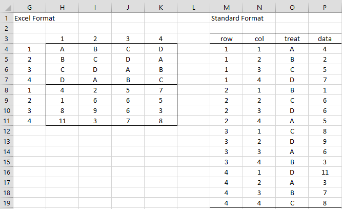
Figure 3 – Latin Squares Design
The linear model of the Latin Squares design takes the form:
![]()
As usual, ∑αi = ∑βj = ∑τk = 0 and εijk∼ N(0,σ2).
Implementation
An Excel implementation of the design is shown in Figure 4.
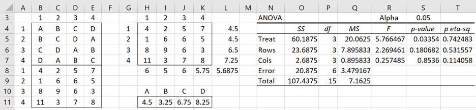
Figure 4 – Latin Square Analysis
The left side of Figure 4 contains the data range in Excel format (equivalent to the left side of Figure 3). The middle part of Figure 4 contains the means of each of the factor levels. Representative formulas used are shown in Figure 5.
| Cell | Factor | Formula |
| L4 | Row | =AVERAGE(H4:K4) |
| H8 | Column | =AVERAGE(H4:H7) |
| H11 | Treatment | =AVERAGEIF($B$8:$E$11,H10,$B$4:$E$7) |
Figure 5 – Formulas for factor means
The right side of Figure 4 contains the ANOVA analysis. The degrees of freedom for all three factors is 3 (cells P4, P5, P6), equal to the number to r – 1, as calculated by =COUNT(B4:B7)-1. dfT = r2 – 1 = 15, while dfE = (r–1)(r–2) = 6.
Formulas for the sum of squares (SS) terms are shown in Figure 6. The other values in Figure 4 are calculated in the usual way.
| Cell | Factor | Formula |
| O5 | Treatment | =DEVSQ(H11:K11)*(P5+1) |
| O6 | Rows | =DEVSQ(L4:L7)*(P6+1) |
| O7 | Columns | =DEVSQ(H8:K8)*(P7+1) |
| O8 | Error | =O9-SUM(O5:O7) |
| O9 | Total | =DEVSQ(H4:K7) |
Figure 6 – Formulas for sums of squares
Results
We see from Figure 4 that there is a significant difference between the four methods (p-value = 0.03345 < .04 = α). There is no significant difference between the operators or between the machines, and so blocking on these factors may not have been necessary in this case.
The analysis is similar when the standard (i.e. stacked) input format is used (see Figure 7). E.g. the mean for row 1 (cell G4) can be calculated by the formula
=AVERAGEIF(A$4:A$19,$F4,$D$4:$D$19
The mean for treatment A (cell I4) can be calculated by using the formula
=AVERAGEIF(C$4:C$19,CHAR($F4+64),$D$4:$D$19)
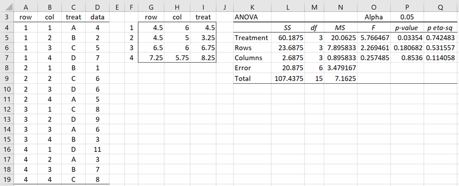
Figure 7 – Latin Square Analysis for stacked format
Observations
In the usual three-factor design, the minimum sample size would be 4 × 4 × 4 = 64, while in this design we only require a sample size of 4 × 4 = 16.
Latin Squares can also be used for a three-factor ANOVA when there are no replications, even when the row and column factors are not nuisance factors, but factors of interest.
Examples Workbook
Click here to download the Excel workbook with the examples described on this webpage.
References
Zhu, M. Y. (2005) Latin square and related design. Statistics 514: Design and Analysis of Experiments, Purdue University
http://www.stat.purdue.edu/~yuzhu/stat514s05/Lecnot/latinsquares05.pdf
Penn State (2025) The Latin Square design
https://online.stat.psu.edu/stat503/lesson/4/4.3
Montgomery, D. C. (2013) Design and analysis of experiments, 8th ed. Wiley
https://faculty.ksu.edu.sa/sites/default/files/douglas_c._montgomery-design_and_analysis_of_experiments-wiley_2012_edition_8.pdf
Hello sir
What should i do when i get my SSE to be zero?
And how do i perform an analysis of the residuals in terms of underlying assumptions of normality, homogenous variance and outliers?
Hello Chantelle,
In general, SSE shouldn’t be zero.
If you email me an Excel spreadsheet with your data and results, I will try to figure out what is happening.
Charles
Can I use excel to get the values of the parameter (overall mean, treatment factor, row factor, column factor)
Hello Ige,
You can get such values, as shown on the webpage.
Charles
what does it mean when you required to construct the ANOVA but SSE =0?
Anton,
SSE = the sum of the squares of the error terms. SSE = 0 means that all the error terms are zero.
E.g. if you made all the rows (or all the columns) in the design the same, then you would get SSE = 0
Why do you ask this question?
Charles
Why the treatment in ANOVA shows #DIV/0 instead of value, I’ve been following the steps above
If you email me an Excel file with your data and the ANOVA results, I will try to figure out why you are getting a division by zero error.
Charles
can you tell me about the factory name which is mentioned in the example .
Please tell me I need that details
Thanu,
Sorry, but the example is fictitious. There is no real factory.
Charles
How to determine the p value? What value that used in that case
You use the same approach as for two factor ANOVA.
Charles
The row average formula in excel should be =AVERAGE(L4:L7), right?
Hello Cody,
I don’t know which row you are referring to, but see Figure 5 for an explanation.
Charles
I’m referring to the row average formula, which is in figure 5. It is the same as the column average formula?
Hi Cody,
Thanks for the clarification and thanks for identifying this error.
As you understood, the formulas should be different. I have now corrected this on the webpage.
I really appreciate your help in improving the accuracy and readability of the website.
Charles
hello sir
How can we perform a Latin square design anova without replication in excel.
Thank you
This webpage shows how to perform Latin Squares design without replication in Excel.
Charles
Dear Sir
I want to compare the performance of two varieties with three replications statistically… Kindly guide me how to add data in excel and which method is to be used for statistical analysis. How two varieties can be compared statistically…
Number of varieties: 2
experiment Place: in pots
Number of replications: 3
if instead of pots we are planting in field then how to analyze. please suggest in both way field/pot.
Thanks
Madhu,
What hypothesis (or hypotheses) do you want to test?
Charles
hello sir my self Mohit Bharadwaj from Allahabad u.p India ,sir want to LSD FORMULA IN EXCLE ,Sir you have a formula plezz mail me- bharadwajmohit1@gmail.com
Mohit,
There isn’t one formula, but the formulas are described on the website.
Charles