Advanced Properties of Probability Distributions

Definition 1: If a continuous random variable x has frequency function f(x) then the expected value of g(x) is

Property 1: If g and h are independent then

Proof: Similar to the proof of Property 1b of Expectation

Definition 2: If a random variable x has frequency function f(x) then the nth moment  M_n(x₀) of f(x) about x₀ is

We also use the following symbols for the nth moment around the origin, i.e. where x₀ = 0

The mean is the first moment about the origin.

We use the following symbols for the nth moment around the mean

The variance is the second moment about the mean

Definition 3: The moment-generating function of a discrete random variable x with frequency function f(x) is a function of a dummy variable θ given by

The moment-generating function for a continuous random variable is

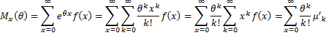
Property 2: If the moment generating function of x for frequency function f(x) converges for each k, then

Proof: We provide the proof where x is a discrete random variable. The continuous case is similar.

Since in general,

it follows that

Thus, the k+1^th term in the power series expansion of the moment-generating function is

The result now follows by induction on k.

Theorem 1: A distribution function is completely determined by its moment-generating function. I.e. two distribution functions with the same moment generating function are equal.

Corollary 1: If x is a random variable that depends on n with frequency function f_n(x) and y is another random variable with frequency function g(x), then if

then

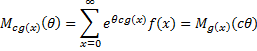
Definition 4: If x is a discrete random variable with frequency function f(x), then the moment generating function of g(x), is

The equivalent for a continuous random variable x is

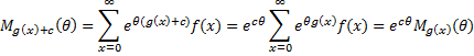
Properties 3: Where c is a constant and g(x) is any function for which M_g(x)(θ) exists

Proof: We prove the property where x is a discrete random variable. The situation is similar where x is continuous.

Property 4: The moment-generating function of the sum of n independent variables is equal to the product of the moment-generating functions of the individual variables; i.e.

Proof: Since the x_i are independent, so are the , and so by Property 2

Theorem 2 (Change of variables technique): If y = h(x) is an increasing function and f(x) is the frequency function of x, then the frequency function g(y) of y is given by

Proof: Let G(y) be the cumulative distribution function of y, let h^-1 be the inverse function of h, and let u = h^-1 (t). Then

Thus

Now by changing variable names, we have

where x = h^-1 (y) and so y = h(x).

Corollary 2: If y = h(x) is a decreasing function and f(x) is the frequency function of x, then the frequency function g(y) of y is given by

Corollary 3: If z = t(x, y) is an increasing function of y, keeping x fixed, and f(x, y) is the joint frequency function of x and y, and h(x, z) is the joint frequency function of x and z, then

Proof: If z = t(x, y) is an increasing function of y, keeping x fixed, and g(y|x) is the frequency function of y|x, and k(z|x) is the frequency function of z|x), then by the theorem

Now let f(x, y) be the joint frequency function of x and y. Then f(x, y) = f(x) · g(y|x). Similarly, if h(x, z) is the joint frequency function of x and z, we have h(x, z) = h(x) · k(z|x). Thus

Since both f and h are the pdf for x, f(x) = h(x), and so we have

Corollary 4: If z = t(x, y) is a decreasing function of y, keeping x fixed, and f(x, y) is the joint frequency function of x and y, and h(x, z) is the joint frequency function of x and z, then

Example 1: Suppose x has pdf f(x) = e^-x where x ≥ 0, and y =. Find the pdf g of y

Since is an increasing function, where x = y², we get

Example 2: Suppose x has pdf f(x) = e^-x for x > 0 and y has pdf g(x) = e^-y for y > 0, and suppose that x and y are independently distributed. Define z = y/x. What is the pdf for z?

From Corollary 3, for fixed x > 0, z = y/x is increasing (since y > 0), and so we have

But since x and y are independently distributed,

Combining the results,

and so

Let w = x(1+z). Then x = w/(1+z). and dx = dw/(1+z). It now follows that

Example 3: Suppose x has standard normal distribution N(0, 1). What is the pdf of the random variable z = |x| and what is the mean of this distribution?

By Definition 1 of Basic Characteristics of the Normal Distribution, the pdf of x is (with μ = 0 and σ = 1)

and so the probability distribution function is

Now |x| < a is equivalent to –a < x < a, and so we have the following formula for z’s distribution function G(z):

Since the pdf g(z) is the derivative of G(z), it follows that

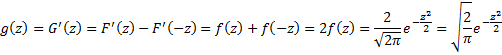
We next use the following using the substitution

and so

Since z ≥ 0, we have

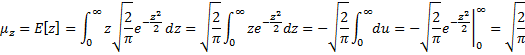
Property 5: If x ~ N(0, σ²), then the mean of |x| is

Proof: Let z = |x/σ|. Thus z ~ N(0, 1), and so as we saw in Example 3, E[z] = . But z = |x|/σ, and so |x| = σz, from which it follows that E[|x|] = .

References

Soch, J. (2020) Proof: Moment-generating function of the normal distribution. The book of statistical proofs
https://statproofbook.github.io/P/norm-mgf.html

Hoel, P. G. (1962) Introduction to mathematical statistics. Wiley