QR Factorization

Definition 1: A QR factorization (or QR decomposition) of a square matrix A consists of an orthogonal matrix Q and an upper triangular matrix R such that A = QR.

Property 1 (QR Factorization): For any n × n invertible matrix A, we can construct a QR factorization.

Proof: Let A₁, …, A_n represent the columns of A. Since A is invertible, we know that A₁, …, A_n are independent and forms a basis for the set of all n × 1 column vectors. We can therefore we can use the Gram-Schmidt process to construct an orthonormal basis Q₁, …, Q_n for the set of all n × 1 column vectors. Let Q be the n × n matrix whose columns are Q₁, …, Q_n. By Property 4 of Orthogonal Vectors and Matrices, Q is an orthogonal matrix, and so by Property 6 of Orthogonal Vectors and Matrices, Q^TQ = I.

We seek a matrix R such that A = QR. Since Q^TQ = I, it follows that Q^TA = Q^TQR = R, and so we conclude that R = Q^TA is the required matrix. Let R = [r_ij], and so r_ij = Q_i · A_j. As we saw in the proof of Theorem 1 of Orthogonal Vectors and Matrices, each Q_i can be expressed as a linear combination of A₁, …, A_i, which means that r_ij = 0 for i > j, which shows that R is an upper triangular matrix. It is also easy to show by induction that r_ij > 0 for each i.

Observation: We can extend Property 1 to certain non-square matrices. The proof is similar and Q and R are constructed in the same way.

Property 2 (QR Factorization): For any m × n matrix A with rank (A) = n ≤ m , we can construct an m × n orthonormal matrix Q and an n × n upper triangular matrix R such that A = QR.

Example 1: Find a QR Factorization for the matrix A that is formed from the columns in Example 1 of Orthogonal Vectors and Matrices.

As can be seen in Figure 1 of Orthogonal Vectors and Matrices, A is a 4 × 3 matrix. The supplemental array formula =ELIM(A4:E7) produces a 4 × 3 matrix with only one zero row showing that rank(A) = 3 (see Appendices Determinants and Linear Equations and Linear Independent Vectors for details). Since rank(A) = 3 ≤ 4, we can apply Property 2.

The orthonormal matrix Q is calculated in Example 1 of Orthogonal Vectors and Matrices. The matrix R = Q^TA is shown in range M4:O6 of Figure 1 of Orthogonal Vectors and Matrices, as calculated using the array formula =MMULT(TRANSPOSE(I4:K7),A4:C7). Note that R is indeed an upper triangular matrix.

Observation: Shortly we will show how to use the QR Factorization to calculate eigenvalues and eigenvectors, and in fact, we will show a better way to produce such a QR Factorization, which is less prone to rounding errors.

For now, we show how to use QR factorization to find the solution to AX = C, the problem studied in Determinants and Linear Equations. First we note that since A = QR and Q is orthogonal, if AX = C, then C = AX = QRX and so Q^TC = Q^TQRX = RX. Thus RX = Q^TC. But since R is an upper triangular matrix all of whose diagonal elements are non-zero (actually they are positive), we can use backwards substitution to find the solution for X. In fact if R =[r_ij], X = [x_j] and Q^TC = [b_i], then we will have a series of equations of the form (looking from the bottom up):

The first equation can be used to find the value of x₁. Substituting this value for x₁ in the second equation enables you to find x₂. Continuing in this manner you can find x_n-1. Substituting these values in the last equation enables you to find x_n.

Example 2: Solve the following system of linear equations using QR Factorization

We could solve this problem using Gaussian elimination, as can be seen from Figure 2 where the array formula =ELIM(U4:X7) in range U10:X13 produces the solution x = -0.34944, y = 0.176822 and z = 0.792727.

Figure 1 – Solving  AX = C using QR Factorization

We now show how to find a solution using QR factorization. First we calculate Q^TC (range Z4:Z6) as =MMULT(TRANSPOSE(I4:K7),X4:X7) using the values for Q shown in Figure 1 of Orthogonal Vectors and Matrices. We next calculate the values for X (range AB4:AB6) via backwards substitution using the formulas in Figure 2.

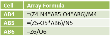
Figure 2 – Formulas in Figure 1

Definition 2: A Householder matrix A is a square matrix for which there exists a vector V such that V^TV = I and A = I – 2VV^T.

Property 3: A Householder matrix is orthogonal

Proof: Let A be a Householder matrix. First we show that A is symmetric, as follows:

We next show that A² = I, from which it follows that AA^T = A² = I, which by definition means that A is orthogonal.

Observation: In Orthogonal Vectors and Matrices, we how to generate a QR factorization for any matrix using the Gram-Schmidt procedure. Unfortunately, for practical purposes, this procedure is unstable, in the sense that as it is applied on a computer, round off errors accumulate and so while theoretically a valid QR factorization is obtained, in practice the results can sometimes be wrong.

We now present a procedure for constructing a QR factorization, using Householder matrices, which is more stable. As we did previously, we start with the case of a square matrix.

Property 4: Every invertible square matrix A has a QR factorization. Furthermore, there is an efficient algorithm for finding this QR factorization.

Define V_k = [v_i] by

v_i = 0 for i < k

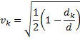
Define P_k = I – 2V_kV_k^T, Q_k = P_kQ_k-1 and R_k+1 = P_kR_k.

Now define R = R_n and Q = Q_n-1^T.

Observation: Property 4 holds even when the square matrix A is not invertible. The proof requires a little tweaking of the procedure described above.

Definition 3: The QR factorization procedure for finding the eigenvalues/vectors of a square matrix is as follows:

Let Q and R be defined as above. Let A₀= A,  Q₀= Q and R₀ = R. Define A_k+1 = R_kQ_k. Since A_k+1 is also invertible it has a QR decomposition A_k+1 = Q_k+1R_k+1.

Property 5: If the eigenvalues of A are distinct and non-zero then A_k converges to an upper triangular matrix with the same eigenvalues as A. If A is symmetric then A_k converges to a diagonal matrix with the same eigenvalues as A.

Observation: Since the eigenvalues of an upper triangular matrix are found on the diagonal, this means that for k sufficiently large the eigenvalues of A are found on the diagonal of A_k.

Example 3: Use the QR decomposition method to find the eigenvalues of 

We begin by finding Q and R.

Figure 3 – QR Factorization using a Householder matrix (step 1)

Thus

where A  = QR, R is an upper triangular matrix and Q^TQ = I. Calling A₀ = A, R₀ = R and Q₀ = Q, we now define a new A = RQ (i.e. A₁ = R₀Q₀) and repeat the process.

Figure 4 – QR Factorization using a Householder matrix (step 2)

The result is a new R and Q, which we now call R₁ and Q₁ such that A₁ = Q₁R₁, R₁ is an upper triangular matrix and Q₁^TQ₁ = I. As before we now define a new A, i.e. A₂ = R₁Q₁ and repeat the process. We continue this process until we get an A_k which is sufficiently close to being a diagonal matrix.

We now skip to the 9th iteration where A has now converged to a diagonal matrix:

Figure 5 – QR Factorization using a Householder matrix (step 9)

Thus

and so

Thus the eigenvalues of the original matrix A are 4, 1 and 1.

Once you find an eigenvalue you can use the Gaussian Elimination Method to find the corresponding eigenvectors since these are solutions to the homogeneous equation (A – λI) X = 0, which can be solved as described in Definition 5 of Determinants and Linear Equations. The only problem with this approach is when the eigenvalues of a matrix are not all distinct (such as in Example 3). Gaussian elimination can find one such eigenvector, but not a set of orthogonal eigenvectors (one for each instance of the repeated eigenvectors, as is required in Example 3).

A better approach is to use the fact that the corresponding eigenvectors are the columns of the matrix B = Q₀Q₁…Q_k (where k is the iteration where A_k is sufficiently close to a diagonal matrix). For Example 3 we define B₀ = Q₀ and B_n+1 = B_nQ_n (shown as B′Q in K32:M34 of Figure 4 and K214:M216 of Figure 5. Thus we conclude that the eigenvectors corresponding to 4, 1, 1 are the columns in the matrix

Since the process described above is complicated and tedious to carry out, it is simpler and faster to use the following Real Statistics functions eigVAL, eigVECT and related functions, as described in Eigenvalues and Eigenvectors.

Example 4: Use the eigVECTSym function to find the eigenvalues and eigenvectors for Example 3.

The output from eigVECTSym(A6:C8) is shown in Figure 6.

Figure 6 – Eigenvalues/vectors using eigVECTSym

which is the same result we obtained previously.

Observation: We can extend Property 4 to certain non-square matrices. The proof is similar and Q and R are constructed in the same way.

Property 6 (QR Factorization): For any m × n matrix A with rank(A) = n ≤ m, we can construct in an efficient way an m × n orthonormal matrix Q and an n x n upper triangular matrix R such that A = QR.

Since the process described above is complicated and tedious to carry out, it is simpler and faster to use the following supplemental functions to create a QR factorization of a matrix.

Real Statistics Functions: The Real Statistics Resource Pack provides the following array functions, where R1 is an m × n range in Excel

QRFactorR(R1, prec): outputs the n × n array R for which A = QR where A is the matrix in R1. 

QRFactorQ(R1, prec): outputs the m × n array R for which A = QR where A is the matrix in R1.

QRFactor(R1, prec): outputs an m+n × n array. The first m rows of the output consist of Q and the next n rows of the output consist of R where A = QR and A is the matrix in range R1.

prec can be used to specify what is considered to be zero in the algorithm used to calculate these functions. The default is 0, but it may be acceptable to use some other small value (e.g. 0.00001) as sufficiently small to be considered to be zero. 

Note that to obtain Q when Property 6 holds, you can also use the fact that Q = AR^-1, and so Q can be obtained via =MMULT(R1, MINVERSE(R2)) where R2 contains the formula =QRFactorR(R1).

Example 5: Find the QR factorization of the matrix in A4:D9 of Figure 7.

Figure 7 – QR Factorization

Range F4:I7 contains the array formula =QRFactorR(A4,D9), Range F10:I15 contains =QRFactorQ(A4,D9), although since R is invertible, Q =AR^-1, and so Q can also be obtained using the worksheet formula =MMULT(A4,D9, MINVERSE(F4:I7)). Finally, range K4:N13 contains the formula =QRFactorR(A4,D9).

We see that A = QR from the formula =MMULT(F10:I15,F4:I7) in range F18:I23. From the formula =MMULT(TRANSPOSE(F10:I15),F10:I15) in range K18:N21, we also see that Q^TQ = I, which demonstrates partial orthogonality, since QQ^T ≠ I.

Observation: Property 6 holds no matter what the rank of matrix A is.

For example, in Figure 8 we display the QR factorization of two 3 × 3 square matrices with rank less than 3.

Figure 8 – QR factorization where rank(A) < 3

Click here for more examples of QR factorization, including the distinction between full and reduced QR factorization and the case where the number of rows in the matrix is less than the number of columns.

Real Statistics Functions: As we saw in Example 2, QR Factorization can be used to solve a system of linear equations. The approach described above can be extended to invert a matrix. The Real Statistics Resource Pack provides the following two functions to automate these processes.

QRSolve(R1, R2) – assuming R1 is an m × n range describing matrix A and R2 is an m × 1 range describing the column vector C, QRSolve outputs an n × 1 column vector X containing the solution to AX = C

QRInverse(R1) = inverse of the matrix described by range R1 (assumes that R1 is a square matrix)

Observation: Referring to Figure 1, QRSolve(U4:W7, X4:X7) would output the result described in AB4:AB7.

Example 6: Find the inverse of the matrix in range W18:Y20 of Figure 9 using QRInverse.

Figure 9 – Matrix inversion using QR Factorization

Using QRInverse(W18:Y20), you obtain the results shown in range AA18:AC20. This is the same result as obtained using MINVERSE(W18:Y20).

Real Statistics Data Analysis Tool: The Matrix data analysis tool contains a QR Factorization option that computes the QR factorization of the matrix in the Input Range. See Figure 3 of Matrix Operations for an example of the use of this tool.