Real Statistics Support for Logistic Regression

Scope

On this webpage, we provide a more detailed description of the Logistic and Probit Regression data analysis tool. In addition, we describe some worksheet functions used by the data analysis tool. These functions provide faster processing as well as support for larger data sets than capabilities described elsewhere on the website.

Data Analysis Tool

Real Statistics Data Analysis Tool: In addition to the capabilities provided by the Logistic and Probit Regression data analysis tool as described in Logistic Regression using Newton’s Method and Logistic Regression Functions, users can choose to uncheck the Item by item details in output option on the dialog box (as shown in Figure 1 below).

We can do this for Example 1 of Comparing Logistic Regression Models, by pressing Ctrl-m and selecting the Logistic and Probit Regression option from the Reg tab (or from the Regression dialog box when using the original user interface) and filling in the dialog box that appears as shown in Figure 1.

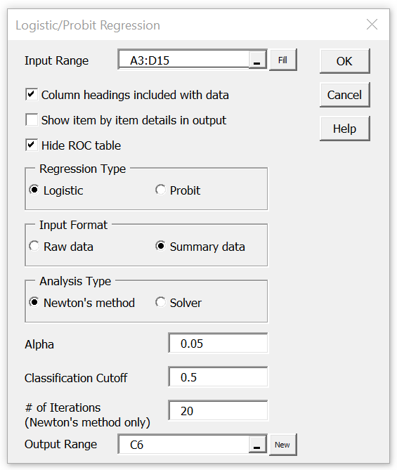
Figure 1 – Logistic and Probit Regression dialog box

When the OK button is pressed, the output shown in Figures 2 and 3 is displayed.

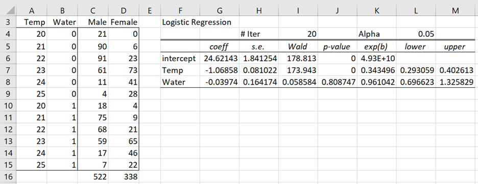
Figure 2 – Logistic Regression analysis (part 1)

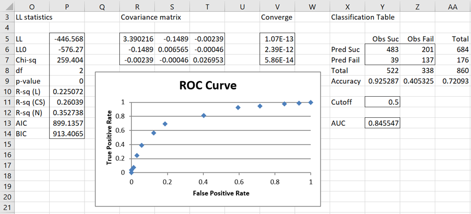
Figure 3 – Logistic Regression analysis (part 2)

The values near zero in column V show that Newton’s method converged to a solution. The p-value of 0 in cell P9 shows that the model is significantly different from the model without independent variables. We see from cell Y13 that this model predicts correctly 84.6% of the 860 observations (based on a cutoff of .5).

The values displayed in Figures 2 and 3 are produced using the following Real Statistics formulas.

Worksheet Functions

Real Statistics Functions:  The following are array functions where R1 contains data in either raw or summary form. Except in the headings, R1 cannot contain any blank or non-numeric entries.

LogitCoeff(R1, lab, raw, head alpha, iter, guess) – calculates the logistic regression coefficients for data in raw or summary form. The output includes the standard errors, Wald statistic, p-value, and 1 – α confidence interval.

lab, raw, head, alpha, iter, and guess are as described in Logistic Regression Functions

For the following functions, R1 is as described above and Rc is a column array containing the logistic regression coefficients for the data in R1.

LogitCov(R1, Rc) – returns the covariance matrix corresponding to the regression coefficients in Rc based on the data in R1.

LogitConverge(R1, Rc,) – returns the F column array described in Property 1 for Newton’s method in Logistic Regression using Newton’s Method. The values in this array should all be close to zero if Rc provides a sufficiently accurate representation of the logistic regression coefficients. Note that if array B adequately represents the true regression coefficients and C represents the covariance matrix for these coefficients (e.g. as calculated by the LogitCov array function) then per Property 2 of Logistic Regression using Newton’s Method, B – CF should be very close to zero.

LogitLL(R1, Rc, lab) – returns a column array with the values LL, LL0, chi-square test results (chi-square stat, df, and p-value), R-square (McFadden, Cox and Snell, Nagelkerke versions), AIC and BIC. This function combines the features of LogitTest and LogitRSquare (as described in Logistic Regression Functions) but does not have to calculate the regression coefficients from scratch. If lab = TRUE (default FALSE) then an extra column is appended to the output which contains labels.

LogitCorrect(R1, Rc, lab, cutoff) – returns a classification (confusion) table for the logistic regression model with the coefficients in Rc based on the data in R1 (as described in Classification Table for Logistic Regression). If lab = TRUE (default FALSE) then an extra row and column containing labels are appended to the output. Predicted probability values ≥ cutoff represent successful outcomes (default .5).

LogitROC(R1, Rc, reduced) – returns an ROC table with FPR and TPR values used to create an ROC curve; see below for a description of the reduced argument.

The LogitCoeff2, LogitSummary, LogitPred, and LogitPredC functions, as described in Logistic Regression Functions, can also be used.

Formulas used in the example

The formulas shown in Figure 4 were used to produce the output in Figures 2 and 3 (as well as Figure 5, as described below).

Output	Range	Formula
Coefficients	F5:M8	=LogitCoeff(A3:D15,TRUE,FALSE,TRUE,L4,I4)
LL and related statistics	O5:P14	=LogitLL(A4:D15,G6:G8,TRUE)
Classification table	X5:AA9	=LogitCorrect(A4:D15,G6:G8,TRUE,Y11)
Covariance matrix	R5:T7	=LogitCov(A4:D15,G6:G8)
Convergence vector	V5:V7	=LogitConverge(A4:D15,G6:G8)
AUC	Y13	=LogitAUC(A4:D15,G6:G8)
ROC table	AC6:AD18	=LogitROC(A4:D15,G6:G8,FALSE)

Figure 4 – Key formulas

Note that the formula =LogitCorrect(A4:D15,G6:G8,FALSE,Y11) would produce the output shown in range Y6:AA9. Note too that the ROC chart shown in Figure 3 is built internally into the data analysis tool. Whereas any change that you make to the input data in range A3:D15 will automatically result in a change to all the other values in Figures 2 and 3, this is not true of the ROC chart.

Hide ROC table option

If you want such changes to also be reflected in the ROC chart or you want to see the (x,y) values that produce the chart, you need to uncheck the Hide ROC table option on the dialog box in Figure 1. In this case, the data analysis tool will also produce the ROC table shown in Figure 5, and the ROC (as shown in Figure 3) will be based on the data in Figure 5. Since any changes that you make to the input data in range A3:D15 will automatically be reflected in the values shown in Figure 5, the ROC will also be updated automatically with the correct values.

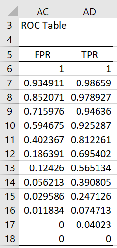
Figure 5 – ROC table

LogitROC reduced argument

The LogitROC function takes reduced as a third argument. If reduced = TRUE (default FALSE) then when R1 has more than 30,000 data elements (actually when the summary version of R1 has more than 30,000 elements when R1 contains raw data), then a reduced form of the ROC table is used. E.g. when there are between 30,000 and 60,000 summary elements, then every other element is used to create the ROC table, Similarly, when there are between 60,000 and 90,000 summary elements, then every third element is used.

Obviously, when there are fewer than 30,000 summary elements then it doesn’t matter which value reduced is set to. Even when the ROC table is reduced, as described, above, the chart should look quite accurate. Note that the data analysis tool internally uses reduced = TRUE when the Hide ROC table option is selected. This is necessary since the ROC chart can’t have more than about 30,000 pairs in this case. When the Hide ROC table option is deselected, then reduced = FALSE is used.

We can perform a similar analysis for data in raw format. When data is in raw format, then we have two choices. The first of these choices is to use the LogitSummary array function to convert the data from raw format to summary format and then use the Logistic and Probit Regression data analysis tool, using the summary data as input, as described above.

The other choice is to use the Logistic and Probit Regression data analysis tool, selecting the Raw data option in Figure 1 and inserting the range containing the raw data in the Input Range, which for Example 1 of Comparing Logistic Regression Models will contain 860 rows plus optionally one column headings row. The output will be identical to that shown in Figures 2 and 3 (and optionally Figure 5).

Examples Workbook

Click here to download the Excel workbook with the examples described on this webpage.

References

Howell, D. C. (2010) Statistical methods for psychology (7^th ed.). Wadsworth, Cengage Learning.
https://labs.la.utexas.edu/gilden/files/2016/05/Statistics-Text.pdf

Christensen, R. (2013) Logistic regression: predicting counts.
http://stat.unm.edu/~fletcher/SUPER/chap21.pdf

Wikipedia (2012) Logistic regression
https://en.wikipedia.org/wiki/Logistic_regression

Agresti, A. (2013) Categorical data analysis, 3rd Ed. Wiley.
https://mybiostats.files.wordpress.com/2015/03/3rd-ed-alan_agresti_categorical_data_analysis.pdf