We now turn our attention to the situation where we use regression with seasonal data: hourly, weekly, monthly, quarterly, etc. For hours we have 24 periods in a day, for months we have 12 periods in a year, etc. In particular, we are concerned with cases where the seasons influence the trend of the data (e.g. annual sales revenues are increasing, but revenues in June are lower than in September).
Example
Example 1: Company XYZ’s quarterly revenues for 2012 through 2015 are shown in column C of Figure 1. We would like to forecast the quarterly revenues for 2016 based on a linear regression model.
As we see from the blue curve in Figure 2, although the annual trend of the revenues may be linear, the graph is certainly not linear due to seasonal fluctuations. We need a way to handle these seasonal fluctuations.
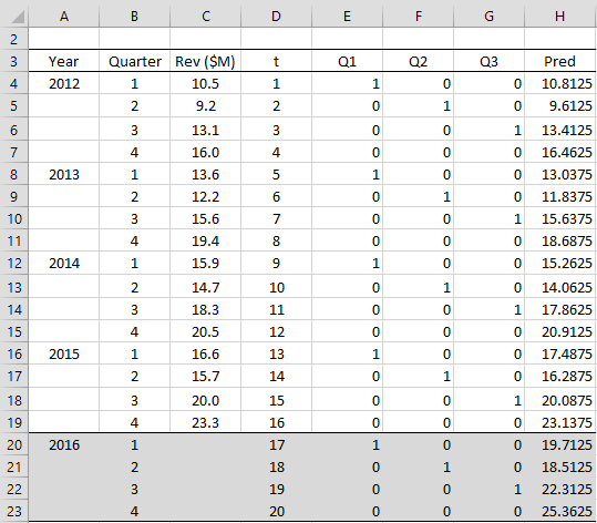
Figure 1 – Seasonal forecasting
Seasonal Approach
The approach we use is to add categorical variables to represent the four seasons (Q1, Q2, Q3, Q4). Three dummy variables are required (one fewer than the number of periods). The coding based on these variables is shown in columns E, F, and G of Figure 1. Column E contains a 1 for revenue data in Q1 and a 0 for revenue data not in Q1. Similarly, column F contains a 1 for data in Q2 and a 0 for data not in Q2. Column G codes for data in Q3. Revenue data in Q4 will have a 0 in columns E, F, and G.
We also include a variable t in column D which simply lists the time periods sequentially ignoring the quarter.
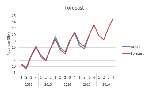
Figure 2 – Seasonal Trends
We now construct a multiple linear regression model using the data in range D3:G19 as our X values and range C3:C19 as our Y values. This analysis is shown in Figure 3.
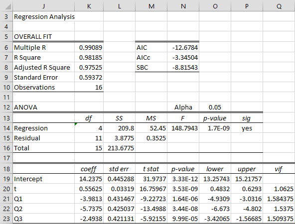
Figure 3 – Regression Analysis with Seasonality
We can use this model to create predictions for the historical data in 2012-2015 as well as for 2016 (future forecast). These predictions are shown in column H of Figure 1 using the array formula
=TREND(C4:C19,D4:G19,D4:G23)
This is the red curve in Figure 2. E.g. the prediction for Q1 of 2012 is $10,812,500 (cell H4), which is fairly close to the actual revenue of $10,500,000 (cell C4).
The forecasted values for each quarter in 2016 are shown in range H20:H23 of Figure 1.
Examples Workbook
Click here to download the Excel workbook with the examples described on this webpage.
Reference
Hansen, B. (2014) Seasonal dummy model
https://users.ssc.wisc.edu/~behansen/390/390Lecture14.pdf
Why did you use 123467… instead od 123412341234? Wouldnt it help alghoritm more?
Hello Peter,
Column B contains 12341234… capturing seasonality, while column D contains 123456… capturing linear trend.
Charles
What if we make intercept = 0. Would that be wrong?
Hello Roman,
You can set the intercept to zero by using Regression through the Origin (aka regression with zero intercept), but is there a reason why you want to do this?
Charles
Hello Charles,
Thank you for the reply. I simply saw such a way on this webpage (https://asmquantmacro.com/2015/06/29/testing-for-seasonality-in-excel/). I guess the author did so in order to select all months (rather than 11 months). If we estimate the model using for instance feb to dec with intercept then the coefficient estimates how much higher or lower returns are in the other months OVER the jan returns. But I guess the goal of the author was to see the how coefficients explain each month’s effect on returns not comparing to jan. So i just wanted to ask if this is also a valid way of capturing seasonality.
Hello Roman,
The regression analysis on this site uses all 12 months but omits an intercept term. This is equivalent to 11 months plus an intercept term.
Charles
Hi all,
How can I make a forecast that is not only based on seasonality but also macro variables?
Thank you!
Hello,
There are a number of approaches. You can use the approach described on this webpage and just include the macro variables. This is ok provided these variables also vary by season. Another approach is to use Panel Analysis. See
https://www.real-statistics.com/panel-data-models/
Charles
Thanks Charles,
For demand forecasting for a certain products with 5 years historical data 2017-2021 ( the data is recorded by the order from the customer, not daily or monthly)
The question, is it better to do the forecast quarterly or monthly? I am using Holt-Winter and Regression to compare with them after I finished
Important note: demand on Jan 2019 is missing
Hi Mo,
Presumably, you have a lot of historical order data you have. This data could be combined to provide daily, weekly, monthly, quarterly, etc. data (assuming that you have enough data). Whether to forecast quarterly or monthly depends on what your needs are.
Charles
Regarding the missing month of data, you can use interpolation as described at
https://www.real-statistics.com/time-series-analysis/stochastic-processes/handling-missing-time-series-data/
Charles
If there is missing data, for example 10% of missing (non-continuous) daily data out of 365 annual data, how can this be done?
Hello Matteo,
It depends on the details, but see the following describing various techniques for handling missing data.
https://www.real-statistics.com/handling-missing-data/
Charles
Hi can you help me understand how to run regression in this scenario.
In case of a retail chain with seasonality trend in data that can be handled the same way but supposingly there are other factors contributing to the trend like number of stores in each quarter, discounts offered.
So how to handle the data with seasonality as well as other factors. Please help
Just add the data for the other variables (one added column for each variable) as you would for any other regression model.
Charles
Why must you account for seasonality when using multiple linear regression to forecast revenue for a particular quarter?
Doug,
You don’t have to account for seasonality, but the resulting forecast will be more accurate if you do (when there is seasonality). Remember that linear regression is based on linearity and seasonality introduces a non-linear component.
harles
Thanks Charles,
For demand forecasting with 5 years historical data ( the data is recorded by the order even if more than one order in a day)
So, is it better to do the forecast quarterly or monthly?
See my previous email response.
Charles
Thanks Charles,
For demand forecasting with 5 years historical data ( the data is recorded by the order, not daily or monthly)
See my previous email response.
Charles
Is it possible to apply the Prais-Wintsen method to control autocorrelation in situations with seasonality?
Also, how do I match the equation in your example to this generic equation: Yi = b0 + b1 * Xi + b2 * sen (2πXi / L) + b3 * cos (2πXi / L)
Where,
Xi is the temporal trend factor
b1 is the slope of the trend,
b2 and b3 the seasonality coefficients,
L is the periodicity constant (for example, months).
This equation would be for a seasonality for a harmonic, as your example.
Thanks a lot
Real Statistics doesn’t yet support the Prais-Winsten method.
You could treat the equation as the linear equation Yi = b0 + b1 * Xi + b2 * Ui + b3 * Vi where Ui = sin(2πXi/L) and Vi = cos(2πXi/L), but probably you would want to use nonlinear regression.
Charles
Hi. How would you interpret the coefficients of the Q1, Q2, Q3 in the output table. e.g. for every increase in Q1, revenue decrease by 3.98?
Shane,
Suppose the dummy variables are q1, q2, q3 for quarters Q1, Q2, Q3m with Q4 acting as the base. For Q1 you need to consider the case where q1 = 1, q2 = 0 and q3 = 0. In this case, the coefficient for the q1 variable is simply added to the intercept coefficient. For Q2 you need to consider the case where q1 = 0, q2 = 1 and q3 = 0. In this case, the coefficient for the q2 variable is simply added to the intercept coefficient. The situation is similar for Q3. For Q4 ou need to consider the case where q1 = 0, q2 = 0 and q3 = 0. In this case, the intercept coefficient captures the impact of Q4. Thus we see that the q1, q2 and q3 coefficients capture the displacement from the intercept, which acts as the Q4 coefficient
Charles
Is an F-test a one-sided hypothesis test because one only rejects the null hypothesis if the calculated statistic is greater than the tabulated critical value?
Yes
Thanks Charles,
Can you please provide a brief justification for the same. It’d be really helpful.
Not sure what you want me to justify, but see https://real-statistics.com/multiple-regression/multiple-regression-analysis/
Charles
What will be the quadratic time trend and how to set seasonal dummies for monthly?
Please also guide me how to formulate the equation as well
Hello Priya,
Instead of using variables Q1, Q2, Q3 use M1, M2, …, M11 for the months. The coding is as explained at
Categorical Coding for Regression
You can also add the term t^2 to the regression model. Its values are the squares of the t values.
Charles
If I am setting up montly dummies, then which month should be excluded, January or December?
Will there be variance in the regression output?
It doesn’t matter which month you exclude. Some aspects of the regression model will be the same and some different.
Charles
Thank you so much
What if the data is provided in weeks, how would you transform it?
Hi Steven,
Use the same approach as described on the webpage, but now you will need 51 dummy variables, one for each week in the year minus one. If, instead, you mean days in the week, then you need 6 dummy variables, one for each day in the week minus one.
Charles
Hi Charles,
If looking at weeks, is it possible to have 51 dummy variables as there is a limit of 16 variables in Excel.
Thanks in advance!
Katherine,
You can have at least 64 variables using the Real Statistics Regression tool (actually more with some options).
Charles
Hi Charles,
Thanks for this, I have 51 (n-1) weeks nd 3 other variables. I’m getting an error “Input x must have at least two more rows of data than columns.” What can be causing this? When I only include 18 weeks I dont get the same error.
Kathrine,
For any linear regression analysis if you have k independent variables you need to have at least k+2 rows of data. The dummy variables used to model the weeks count towards this value of k.
Charles
Hi Charles!
I’ve got a question about your regression model, y = a+ b * X + error, do we have 4 (one for each Q) or 5 (one for each Q + 1 for ‘quaternumber’).
Thank you very much for this great website!
Ella
Ella,
It depends on what independent variables you put in the model. If say you have 4 seasons, then you need 4-1 = 3 dummy variables to model the seasons. In the example given on the webpage, another variable was used to model the trend (t for time or trend). You might have other independent variables that are not about seasons or time.
Charles
Hi,
How can we calculate the standard deviation of our forecast ?
Thank you,
Hello Hanna,
See https://real-statistics.com/multiple-regression/confidence-and-prediction-intervals/
Charles
I am using linear and log linear regression to review a large amount of products for which I have weekly sales(split into months for the analysis) and the aim is to assign a suitable seasonal pattern for each item. However, I am unclear which of the statistical output of the regression would guide me on whether there is seasonality or not on my data? Should I use an average of the sales index or forecast index produced by the regression or how could I tell if there is no seasonality and I should assume index=1 across all 52 periods?
I wanted to clarify that I have used the Linest function in my data so that I can run Macros on the analysis so I have not got the p values(significance of each variable) shown. I am unsure how to get the p value also in excel as part of that analysis. If you could also help on that it would be great. Many thanks
Hi Dimi,
1. You can create a plot of your data to determine whether there is seasonality. If there is seasonality, you should be able to spot the pattern (monthly, quarterly, etc.).
2. To calculate the p-value for each coefficient, you take the slope value (row 1 from LINEST) and divide it by the standard error (row 2 from LINEST). This yields the t statistic. You can now calculate the p-value for that coefficient using =T.DIST.2T(t,n-2) where n = the sample size.
Charles
Great many thanks for the formula. That will help a lot. Would though a high p(low significance) show that there is no consistent impact for March let’s say if the p for the dummy March variant would be more thank 0.05?Or else what does a high p for that variable (one of the 11 months) would mean I should do different with this month?
Finally would there be an easy way to exclude the impact of the trend from my data to get to an accurate index?
Many thanks again
Dimitra
Hello Dimi,
1. The actual interpretation of each of the coefficients is complicated by the fact that there are also non-seasonality variables. If there are no other variables, the situation is similar to that described at
https://real-statistics.com/multiple-regression/anova-using-regression/
If you want to determine whether seasonality is significant, then you can compare the regression model without the seasonality dummy variables with the model that includes all the seasonality variables by using the approach described at
https://real-statistics.com/multiple-regression/testing-significance-extra-variables-regression-model/
2. Yes, just omit the trend variable from the regression model.
Charles
To capture seasonality, we use dummy variables. What is the rational behind using one less number of variables than the number of periods. For example, for a quarterly data, we add three variables, not four, and for monthly data, we add 11, not 12 variables.
Hello Chaman,
If you use one dummy variable per period, then the values for this variable will be a linear combination of the other variables and the regression will not succeed due to multicollinarity. You can learn more about the coding at
https://real-statistics.com/multiple-regression/multiple-regression-analysis/categorical-coding-regression/
Charles
Hi, can you please mention a detailed article that describes why we use n-1 variables, I still don’t get it
Thanks in advance
Hi Shawky,
If you use n variables, then one of the variables will be a linear combination of the others, in which case you will have multicollinearity and the regression model won’t work. I suggest that you try using n variables and see what happens. Also, see
Collinearity
Charles
My question is that how to predict future after applying multiple regression technique we didn’t able to predict
Musa,
This webpage shows how to predict future events.
Charles
QUESTION FIVE
Sales of article B (’000 units)
QI Q2 Q3 Q4 (Q = quarter)
2015 24.8 36.3 38.1 47.5
2016 31.2 42.3 43.4 55.9
2017 40.0 48.8 54.0 69.1
2018 54.7 57.8 60.3 68.9
(a) Look at the data. What sort of trend and seasonal pattern do you expect to emerge from the analysis of this data? (2 marks)
(b) Derive a regression equation from the data and forecast the trend in sales for the four quarters of 2019 (2 marks)
(c) Discuss the usefulness of this method of forecasting.
(1 mark)
What sort of help do you need?
Charles
How to get the values in M6:N8; that is AIC/AICc and SBC. I dont get these as output while using excel built in function inside Data Analysis–Regression.
Hello Gulshan,
Yes, these values are not available from Excel’s data analysis tool. These values are available from the Real Statistics Regression data analysis tool. You can download the Real Statistics software for free at
Real Statistics Resource Pack
Charles
Hi Please help me to answer this question
Given the following table, forecast for the production of shirt using REGRESSION method for 2019, 2020 and 2021.Show your solution.
YEAR PRODUCTION SALES
2012 343.5 PIECES P12,789 M
2013 381.2 PIECES P4567 M
2014 437.5 PIECES P 12,345 M
2015 323.6 PIECES P 18965 M
2016 231.4 PIECES P76239 M
2017 443.5 PIECES P34897M
2018 525.2 PIECES P23419 M
Hello Lea,
What is your question?
Charles
How would I build the model if there were seasonality but not trend?
There are a few approaches, but the simplest is to use the method described on this webpage. If there is no trend then this will be apparent from the regression coefficients.
Charles
Julybug, time series forecasting includes seasonality, trend, and noise. Thus, you your data must reflect some form of trend component to use uni-variate time series analysis.
My only question is should I use “t” in the regression equation? To me T represents Quarter 4. However, I have heard Quarter 4 is represented in the Y intercept? I am confused.
Should I use the x variable t in the regression equation or leave it out?
Thank you.
Shah,
You need to include the t variable. You can call it whatever you want, but it isn’t Quarter 4.
Charles
What’s the advantage of including “t” as a variable in the model?
In addition to the seasonality, there is an upward trend to the data (see the chart). This is captured by t.
Charles
It’s important to account for a possible time trend.
Since you’re checking for seasonality “t” needs to be included
The main thing the forecast formula is not explained. Doesnt make sense. Can you write the formulaS for forecast cells?
LH,
This webpage builds on concepts described in other webpages. The main concept is to use dummy coding to capture the quarters. This is explained at:
https://real-statistics.com/multiple-regression/multiple-regression-analysis/categorical-coding-regression/
The other concept is regression forecasting using the TREND function. This is explained at:
https://real-statistics.com/multiple-regression/multiple-regression-analysis/multiple-regression-analysis-excel/
Charles
What is the prediction formula for the second period, etc?
Thank you
Steven,
You can use the TREND function as described on the website. E.g. the formula in cell H21 is =TREND(C4:C19,D4:G19,D21:G21)
Charles