Assumptions
In Multiple Regression Analysis, we note that the assumptions for the regression model can be expressed in terms of the error random variables as follows:
- Linearity: The εi have a mean of 0
- Independence: The εi are independent
- Normality: The εi are normally distributed
- Homogeneity of variances: The εi have the same variance σ2
Testing Residuals
If these assumptions are satisfied then the random errors εi can be regarded as a random sample from an N(0, σ2) distribution. It is natural, therefore, to test our assumptions for the regression model by investigating the sample observations of the residuals
![]()
It turns out that the raw residuals ei follow a normal distribution with mean 0 and variance σ2(1-hii) where the hii are the terms in the diagonal of the hat matrix defined in Definition 3 of Method of Least Squares for Multiple Regression. Unfortunately, the raw residuals are not independent.
By Property 3b of Expectation, we know that
![]()
The ri have the desired distribution, but they are still not independent. If, however, the hii are reasonably close to zero then the ri can be considered to be independent. As usual, MSE can be used as an estimate for σ.
Studentized Residuals
Definition 1: The studentized residuals are defined by
![]()
If the εi have the same variance σ2, then the studentized residuals have a Student’s t distribution, namely
![]()
where n = the number of elements in the sample and k = the number of independent variables.
We can now use the studentized residuals to test the various assumptions of the multiple regression model. In particular, we can use the various tests described in Testing for Normality and Symmetry, especially QQ plots, to test for normality, and we can use the tests found in Homogeneity of Variance to test whether the homogeneity of variance assumption is met.
It should also be noted that if the linearity and homogeneity of variances assumptions are met then a plot of the studentized residuals should show a randomized pattern. If this is not the case then one of these assumptions is not being met. This approach works quite well where there is only one independent variable. With multiple independent variables, we need a plot of the residuals against each independent variable. Even then we may not capture multi-dimensional issues.
Example
Example 1: Check the assumptions of regression analysis for the data in Example 1 of Method of Least Squares for Multiple Regression by using the studentized residuals.
We start by calculating the studentized residuals (see Figure 1).

Figure 1 – Hat matrix and studentized residuals
First, we calculate the hat matrix H (from the data in Figure 1 of Multiple Regression Analysis in Excel) by using the array formula
=MMULT(MMULT(E4:G14,E17:G19),TRANSPOSE(E4:G14))
where E4:G14 contains the design matrix X. Alternatively, H can be calculated using the Real Statistics function HAT(A4:B14). From H, the vector of studentized residuals is calculated by the array formula
=O4:O14/SQRT(O19*(1-INDEX(Q4:AA14,AB4:AB14,AB4:AB14)))
where O4:O14 contains the matrix of raw residuals E, and O19 contains MSRes. See Example 2 in Matrix Operations for more information about extracting the diagonal elements from a square matrix.
We now plot the studentized residuals against the predicted values of y (in cells M4:M14 of Figure 2).

Figure 2 – Studentized residual plot for Example 1
The values are reasonably spread out, but there does seem to be a pattern of rising value on the right, but with such a small sample it is difficult to tell. Also, some of this might be due to the presence of outliers (see Outliers and Influencers).
Worksheet Function
Real Statistics Function: The Real Statistics Resource Pack provides the following array function where R1 is an n × k array containing X sample data and R2 is an n × 1 array containing Y sample data.
RegStudE(R1, R2) = n × 1 column array of studentized residuals
Thus, the values in the range AC4:AC14 of Figure 1 can be generated via the array formula RegStudE(A4:B14,C4:C14), again referring to the data in Figure 3 of Method of Least Squares for Multiple Regression
Data Analysis Tool
Real Statistics Data Analysis Tool: The Multiple Linear Regression data analysis tool described in Real Statistics Capabilities for Linear Regression provides an option to test the normality of the residuals.
For Example 2 of Multiple Regression Analysis in Excel, this is done by selecting the Normality Test option on the dialog box shown in Figure 1 of Real Statistics Capabilities for Linear Regression. When you select this option the output shown in range J2:K14 of Figure 3 is displayed. Note that this is the same output that is obtained from the Shapiro-Wilk option of the Descriptive Statistics and Normality data analysis tool on the residuals in range E4:E14 (obtained via the array formula =RegE(A4:B14,C4:C14)).
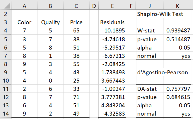
Figure 3 – Normality test of residuals
Examples Workbook
Click here to download the Excel workbook with the examples described on this webpage
References
Howell, D. C. (2010) Statistical methods for psychology (7th ed.). Wadsworth, Cengage Learning.
https://labs.la.utexas.edu/gilden/files/2016/05/Statistics-Text.pdf
Wooldridge, J. M. (2013) Introductory econometrics, a modern approach (fifth edition). Cengage Learning
https://faculty.cengage.com/works/9781337558860
Dear Dr Zaiontz,
Thank you for your great explanations! I am just wondering – i see you provided a way to test linearity, normality and homogeneity of residuals, however how do you test their independence?
Is there something that I’m missing in the text you wrote above?
Thank you so much,
Cristian
Wait, i think i understand, but a confirmation from your side i think would help – the ri’s, by the mathematical way they are constructed are a priori independent (provided that hii are approx. 0), so no need to test this with studentized residuals, right?
Thank you so much,
Cristian
Cristian,
You can test for independence after you have accumulated the data in these sorts of approaches (checking that covariance = 0), and this may be necessary with historical data for example. For (multivariate) normally distributed data, independence is equivalent to covariance = 0.
Generally, though, you ensure independence by conducting your experiment using randomization techniques to make sure that you have a random sample.
Charles
Dear Cristian!
Durbin Watson!
Thanks!
Hello Charles,
I’m trying to implement in Excel the analysis of Example 1 above, starting from the input values of Example 1 in https://real-statistics.com/multiple-regression/least-squares-method-multiple-regression/ (color/quality/price).
However, I’m having trouble calculating the hat matrix H using those input data. Based on your formula above:
=MMULT(MMULT(E4:G14,E17:G19),TRANSPOSE(E4:G14))
I know E4:G14 is the matrix with the input data (A4:C14 in my spreadsheet), but what is E17:G19? I can’t figure it out, and I can’t get the same results as in Figure 1.
Thanks so much!
Hello Enrico,
The matrix in E17:G19 is described on the following webpage
https://real-statistics.com/multiple-regression/multiple-regression-analysis/multiple-regression-analysis-excel/
just below Figure 1.
Charles
Why do we sometimes need to natural log the residual values to get a better model ? Sometimes we have bad residual plot models. Thanks.
Hello,
I don’t know why you need to take the natural log of the residuals. This probably depends on what you plan to do with these residuals.
Charles
Hi Charles,
Hope you are well. Nice to see the website is going strong since inception.
What do you mean or how do you come to the conclusion that – “It turns out that the raw residuals have the distribution” and then the equation with mean 0 and standard deviation, sigma * sqrt(1-value in hat matrix)
I’ve read the use of standardized and studentized residuals to help identify outliers/leverage points that would not normally be detected with raw residuals but not sure I understand what you mean regarding the original distribution of the raw residuals, which led you to use studentized residuals?
Kind regards
Declan
Hello Declan,
The theoretical (population) residuals have desirable properties (normality and constant variance) which may not be true of the measured (raw) residuals. Some of these properties are more likely when using studentized residuals (e.g. t distribution).
Admittedly, I could explain this more clearly on the website, which I will eventually improve. Thanks for your question.
Charles
Thanks man 🙂
Have a good weekend.
Hi Charles, thank you for your website.
Currently I have my regression model of:
LN(COEP) = 22.05 + 0.71 LN(Demand) – 2.31 LN(Quota) + error term
Does error term in regression same as standard deviation? What should I do with the error term? I try to predict my COEP with given demand and quota. However, the predicted COEP is so much different from the observed COEP.
Does anything wrong with my regression model?
Thank you.
Jessica,
The error term is not the standard deviation. It can be viewed as the difference between the actual value of y and the one forecasted by the regression model. When using the regression model for prediction, you can ignore the error term.
If your predicted value is very different from the actual value, this could indicate that the regression model is not a good model for your data. You should draw a chart of each of the independent variables, LN(Demand) and LN(Quota), against the dependent variable, LN(COEP), and see whether these look like they follow a straight line.
Charles
Hello Charles,
Apologies in advance if this is a silly question, but the linked page on Expectation does not have a Property 3b. What section should the link reference?
Thanks once again for the invaluable resource. Your website is often the first place I look when I have a statistics question.
Andrew,
The second of the two statements (the one about variance)
Charles
Can you please explain to me what is the Raw Residual ?
Thanks in advance !
Alhanouf,
The raw residual is e_i on the referenced webpage, i.e. y_i minus the predicted value of y_i.
Charles
Hi, Charles. Thank you for your website. Above, you state: “First we calculate the hat matrix H (from the data in Figure 3 of Method of Least Squares for Multiple Regression) by using the array formula…”. There is no Figure 3 of Method of Least Squares for Multiple Regression.
Regards,
Tara
Tara,
Thanks for catching this mistake. The reference should be to Figure 1 of Multiple Regression Analysis in Excel. I have now corrected the referenced webpage.
Charles