Stepwise Regression

When there are a large number of potential independent variables that can be used to model the dependent variable, the general approach is to use the fewest number of independent variables that can do a sufficiently good job of predicting the value of the dependent variable. This leads to the concept of stepwise regression, which was introduced in Testing Significance of Extra Variables. The reader is once again alerted to the limitations of this approach, as described in Testing Significance of Extra Variables.

In this webpage, we describe a different approach to stepwise regression based on the p-values of the regression coefficients. The algorithm we use can be described as follows where x₁, …, x_k are the independent variables and y is the dependent variable:

0. Establish a significance level. Whereas for most statistical tests a value of alpha = .05 is chosen, here it is more common to choose a higher value such as alpha = .15 or .20.

1a. Build the k linear regression models containing one of the k independent variables. Choose the independent variable whose regression coefficient has the smallest p-value in the t-test that determines whether that coefficient is significantly different from zero. Let’s call this variable z₁ (i.e. z₁ is one of the independent variables x₁, …, x_k) and the p-value for the z1 coefficient in the regression of y on z1 is p.

1b. If p ≥ α. Then stop and conclude there is no acceptable regression model. Otherwise, continue to step 2a.

2a.   Assuming that we have now built a stepwise regression model with independent variables z₁, z₂, …, z_m (after step 1b, m = 1), we look at each of the k–m regression models in which we add one of the remaining k-m independent variables to z₁, z₂, …, z_m. As in step 2a, choose the independent variable whose regression coefficient has the smallest p-value. Let’s call this variable z_m+1 and suppose the p-value for the z_m+1 coefficient in the regression of y on z₁, z₂, …, z_m, z_m+1 is p.

2b.   If p ≥ α. Then stop and conclude that the stepwise regression model contains the independent variables z₁, z₂, …, z_m. Otherwise, continue on to step 2c.

2c.    Now consider the regression model of y on z₁, z₂, …, z_m+1 and eliminate any variable z_i whose regression coefficient in this model is greater than or equal to α.  This leaves us with at most m+1 independent variables. Now loop back to step 2a.

Note that this process will eventually stop. In order to make this process clearer, let’s look at an example.

Example

Example 1: Carry out stepwise regression on the data in range A5:E18 of Figure 1.

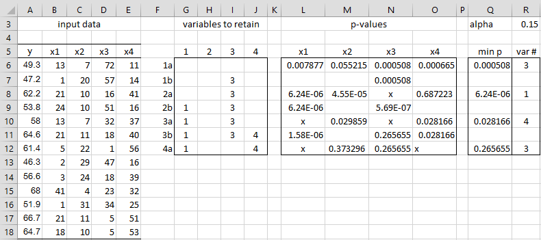
Figure 1 – Stepwise Regression

The steps in the stepwise regression process are shown on the right side of Figure 1. Columns G through J show the status of the four variables at each step in the process. An empty cell corresponds to the corresponding variable not being part of the regression model at that stage, while a non-blank value indicates that the variable is part of the model. We see that the model starts out with no variables (range G6:J6) and terminates with a model containing x₁ and x₄ (range G12:J12).

Columns L through O show the calculations of the p-values for each of the variables. The even-numbered rows show the p-values for potential variables to include in the model (corresponding to steps 1a and 2a in the above procedure). An “x” in one of these cells indicates that the corresponding variable is already in the model (at least at that stage) and so a p-value doesn’t need to be computed.

E.g. the value in cell L6 is the p-value of the x₁ coefficient for the model containing just x₁ as an independent variable. The value in cell L8 is the p-value of the x₁ coefficient for the model containing x₁ and x₃ as independent variables (since x₃ was already in the model at that stage). The values in range L8:O8 are computed using the array worksheet formula =RegRank($B$6:$E$18,$A$6:$A$18,G8:J8), which will be explained below.

For each even row in columns L through O, we determine the variable with the lowest p-value using formulas in columns Q and R. E.g. cell Q6 contains the formula =MIN(L6:O6) and R6 contains the formula =MATCH(Q6,L6:O6,0). Thus we see that variable x₃ is the first variable that can be added to the model (provided its p-value is less than the alpha value of .15 (shown in cell R3). This we test in cell J7 using the formula =IF($R6=J$5,J$5,IF(J6=””,””,J6)).

The odd-numbered rows in columns L through O show the p-values that are used to determine the potential elimination of a variable from the model (corresponding to step 2b in the above procedure). These p-values are calculated using the array formula

=RegCoeffP($B$6:$E$18,$A$6:$A$18,G7:J7)

which we will describe below. A blank value in any of these rows just means that the corresponding variable was not already in the model and so can’t be eliminated.

The determination of whether to eliminate a variable is done in columns G through J. For example, the test as to whether to eliminate the variable x₄ from the model at the second step (when we have just added variable x₁) is done in cell G10 using the formula =IF(L9>=$R$3,””,IF(G9=””,””,G9)). We see that x₁ is not eliminated from the model. In the following step, we add variable x₄ and so the model contains the variables x₁, x₃, x₄). We now test x₁ and x₃ for elimination and find that x₁ should not be eliminated (since p-value = 1.58E-06 < .15), while x₃ should be eliminated (since p-value = .265655 ≥ .15).

In the final step of the stepwise regression process (starting with variables x₁ and x₄), we test variables x₂ and x₃ for inclusion and find that the p-values for both are larger than .15 (see cells M12 and N12).

Worksheet Functions

Real Statistics Functions: The Stepwise Regression procedure described above makes use of the following array functions. Here, Rx is an n × k array containing x data values, Ry is an n × 1 array containing y data values and Rv is a 1 × k array containing a non-blank symbol if the corresponding variable is in the regression model and an empty string otherwise. If cons = TRUE (default) then regression with a constant term is used; otherwise regression through the origin is employed.

RegRank(Rx, Ry, Rv, cons) – returns a 1 × k array containing the p-value of each x coefficient that can be added to the regression model defined by Rx, Ry, and Rv.

RegCoeffP(Rx, Ry, Rv, cons) – returns a 1 × k array containing the p-value of each x coefficient in the regression model defined by Rx, Ry, and Rv.

We can also determine the final variables in the stepwise regression process without going through all the steps described above by using the following array formula:

RegStepwise(Rx, Ry, alpha, cons) – returns a 1 × k array Rv where each non-blank element in Rv corresponds to an x variable that should be retained in the stepwise regression model. Actually, the output is a 1 × k+1 array where the last element is a positive integer equal to the number of steps performed in creating the stepwise regression model. alpha is the significance level (default .15).

Data Analysis Tool

Real Statistics Data Analysis Tool: We can use the Stepwise Regression option of the Linear Regression data analysis tool to carry out the stepwise regression process.

For example, for Example 1, we press Ctrl-m, select Regression from the main menu (or click on the Reg tab in the multipage interface), and then choose Multiple linear regression. On the dialog box that appears (as shown in Figure 2.

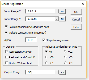
Figure 2 – Dialog box for stepwise regression

The output looks similar to that found in Figure 1, but in addition, the actual regression analysis is displayed, as shown in Figure 3.

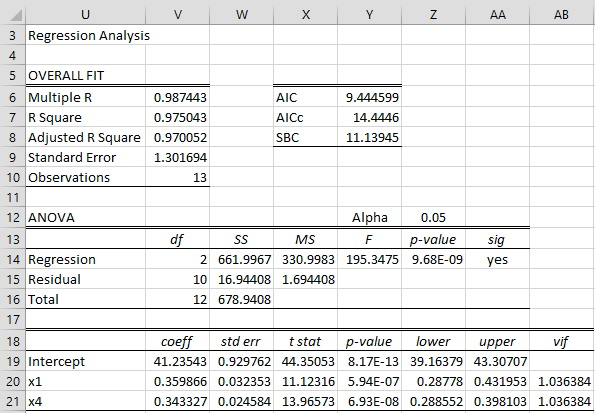
Figure 3 – Stepwise Regression output

Note that the SelectCols function is used to fill in some of the cells in the output shown in Figure 3. For example, the range U20:U21 contains the array formula =TRANSPOSE(SelectCols(B5:E5,H14:K14)) and range V19:W21 contains the array formula =RegCoeff(SelectCols(B6:E18,H14:K14),A6:A18). Here the range H14:K14 describes which independent variables are maintained in the stepwise regression model. This range is comparable to range H12:K12 of Figure 1 and contains the same values.

If the Include constant term (intercept) option is checked on the dialog box in Figure 2 then regression with a constant is used; otherwise, regression through the origin is employed.

Reference

Penn State University (2016) Stepwise regression
https://online.stat.psu.edu/stat501/lesson/10/10.2