Correspondence Analysis Basic Concepts

Overview

Correspondence analysis plays a role similar to factor analysis or principal component analysis for categorical data expressed as a contingency table (e.g. as described in the chi-square test of independence). For a 10 × 10, a complete description of the associations between row elements and column elements requires nine dimensions. Unfortunately, it is difficult for us to visualize such associations in more than two dimensions. In correspondence analysis, we project the row/column associations into two dimensions even if this requires that there is some loss in the accuracy of the representation.

Essentially, correspondence analysis decomposes the chi-square statistic of independence into orthogonal factors. This approach is valid even when the cell sizes in the contingency table are less than 5 (or even zero).

Examples

Example 1: 80 teenagers were asked to select which of 6 characteristics best describe 4 popular brands of smartphones. The teenagers were permitted to comment on multiple brands of smartphones and choose more than one characteristic of any of the brands.

The brands are Apple, Samsung, Nokia, and Huawei. The characteristics are Screen Display, Price, Design, Battery, Software, and Camera. The raw data is shown in Figure 1.

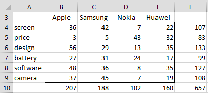
Figure 1 – Survey data

Note that the chi-square statistic for this contingency table is 164.33, as calculated, for example, by the Real Statistics formula =CHI_STAT(B4:E9). The inertia statistic is now set to the chi-square statistic divided by the sample size, i.e. 164.33/657 = .2501.

Proportional Matrix

We next create the proportional matrix P by dividing each of the elements in the contingency table by the sample size, as shown in range O3:S9 of Figure 2.

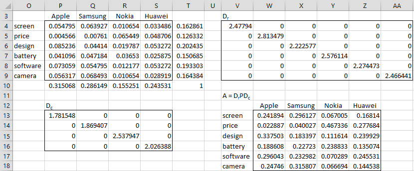
Figure 2 – Proportional matrix

Next, we create the row totals in range T4:T9 and column totals in range P10:S10, and then the 6 × 6 array D_r (in range V4:AA9) using the array formula

=DIAGONAL(1/SQRT(T4:T9))

Here DIAGONAL(R1) is the Real Statistics array function that outputs a diagonal matrix whose diagonal consists of the elements in the row or column range R1, which in this case consists of the reciprocal of the square root of the elements in range T4:T9. Similarly, we create the 4 × 4 array D_c (located in range P13:S16) using the array formula =DIAGONAL(1/SQRT(P10:S10)).

Single Value Decomposition

We now create matrix A = D_rPD_c, as shown in range W13:Z18, using the array formula =MMULT(V4:AA9,MMULT(P4:S9,P13:S16)). Finally, we used the Matrix Operations data analysis tool to create a singular value decomposition of matrix A, as shown in Figure 3.

Figure 3 – Singular Value Decomposition

We now calculate the F and G coordinate matrices and DD^T matrix as shown in Figure 4. The coordinate matrices contain the factor coordinates and the DD^T matrix contains the eigenvalues that are used to decompose the chi-square statistic.

Figure 4 – Coordinate matrices and eigenvalues

Eigenvalues

From the DD^T matrix, we obtain the Eigenvalue table shown in Figure 5. This table corresponds to the table that produces a scree plot for factor analysis. In fact, we can use the table to create a scree plot for correspondence analysis. With just three potential factors, we won’t actually create the scree plot for this example.

Figure 5 – Eigenvalue decomposition

This table tells us that the first factor accounts for 87.57 % of the variation and the second factor accounts for 10.56% of the variation. Consequently, the first two factors account for 98.13% of the variation, and so we only lose 1.43% of the variation if we use only these two factors.

Note that the sum of the eigenvalues (i.e. the trace), 0.2501, is equal to the inertia that we calculated earlier (just after Figure 1).

A rule of thumb is that a two-dimension correspondence analysis (i.e. one where we retain just two factors) is sufficient, provided the first two eigenvalues account for at least 50% of the variation, ideally much more. If this rule of thumb is not met, then we need to make a trade-off between adding more factors and the difficulty of visualizing the information when more than two dimensions are used. For our purposes, we will assume that two factors are sufficient.

Correspondence Analysis Plot

We next create the correspondence analysis plot detail reports for rows and columns, as shown in Figure 6.

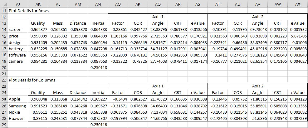
Figure 6 – Plot Detail Reports

Since we retain two factors, we use two dimensions (or axes) in each report. Figure 7 describes the screen display profile entries in the Rows report (row 14).

Figure 7 – Detailed description of screen display profile

The description of the axis 2 components of the screen display profile is similar to the axis 1 descriptions shown in Figure 7, except that now the next column of the F matrix is used (i.e. range AE12:AE17 of Figure 4).

Note that cell AN20 contains the total inertia, as calculated by the formula =SUMPRODUCT(AL25:AL28,AM25:AM28). Note that this value, .2501, agrees with the value that we calculated twice previously.

The values in the Column part of the report in Figure 6 are calculated as described in Figure 7, except that now we use the factors that result from the columns in the G matrix of Figure 4.

The row profile coordinates that are most important are characterized by COR > 1/k and CTR > 1/r where r = # of rows, c = # of columns, and k = min(r, c) – 1. For Example 1 r = 6, c = 4, and k = 3, and so the most important row coordinates are characterized by COR > .3333 and CTR > .1667, which means that the most important row coordinates are for factor 1 of price and factor 2 of design and battery.

Similarly, the most important column profile coordinates are characterized by COR > 1/k and CTR > 1/c.

References

Hintze, J. L. (2007) Correspondence analysis. NCSS.
https://www.ncss.com/wp-content/themes/ncss/pdf/Procedures/NCSS/Correspondence_Analysis.pdf

Garson, G. D. (2012). Correspondence Analysis. Asheboro, NC: Statistical Associates Publishers.

Yelland, P. M. (2010) An introduction to correspondence analysis. The Mathematica Journal
https://www.mathematica-journal.com/2010/09/20/an-introduction-to-correspondence-analysis/