Tukey HSD (Honestly Sig Diff) | Real Statistics Using Excel

Basic Concepts

The idea behind the Tukey HSD (Honestly Significant Difference) test is to focus on the largest value of the difference between two group means. The relevant statistic is

where n = the size of each of the group samples. The statistic q has a distribution called the studentized range q (see Studentized Range Distribution). The critical values for this distribution are presented in the Studentized Range q Table based on the values of α, k (the number of groups), and df_W. If q > q_crit then the two means are significantly different.

This test is equivalent to

Picking the largest pairwise difference in means allows us to control the experiment-wise error rate for all possible pairwise contrasts; in fact, Tukey’s HSD keeps experiment-wise α = .05 for the largest pairwise contrast and is conservative for all other comparisons.

Note that the statistic q is related to the usual t statistic by q = $\sqrt 2$ t. Thus we can use the following t-statistic

Critical value and confidence interval

The critical value for t is now given by t_crit = q_crit / $\sqrt 2$ . If t > t_crit then we reject the null hypothesis that H₀: μ_max = μ_min, and similarly for other pairs.

As described above, to control type I error, we can’t simply use the usual critical value for the distribution, but instead, use a critical value based on the largest difference of the means.

From these observations we can calculate confidence intervals in the usual way:

or equivalently

Example

Example 1: Analyze the data from Example 3 of Planned Comparisons using Tukey’s HSD test to compare the population means of women taking the drug and the control group taking the placebo.

Using the Studentized Range q Table with α = .05, k = 4, and df_W = 44, we get q_crit = 3.7775. Note that since there is no table entry for df = 44, we need to interpolate between the entries for df = 40 and df = 48. Alternatively, we can employ Excel’s table lookup capabilities. We can also use the Real Statistics function QCRIT(4,44,.05,2,FALSE), as described below, to get the same result of 3.7775.

The critical value for differences in means is

Since the difference between the means for women taking the drug and women in the control group is 5.83 – 3.83 = 1.75 and 1.75 is smaller than 1.8046, we conclude that the difference is not significant (just barely). The following table shows the same comparisons for all pairs of variables:

Figure 1 – Pairwise tests using Tukey’s HSD for Example 1

From Figure 1 we see that the only significant difference in means is between women taking the drug and men in the control group (i.e. the pair with the largest difference in means). We can also use the t-statistic to calculate the 95% confidence interval as described above. In Figure 2 we compute the confidence interval for the comparison requested in the example as well as for the variables with maximum difference.

Figure 2 – Tukey HSD confidence intervals for Example 1

Worksheet Functions

Real Statistics Function: The following function is provided in the Real Statistics Resource Pack:

QCRIT(k, df, α, tails, h) = the critical value of the Studentized range q for k independent variables, the given degrees of freedom and value of alpha, and tails = 1 (one tail) or 2 (two tails, default). If h = TRUE (default) harmonic interpolation is used; otherwise, linear interpolation is used.

QPROB(q, k, df, tails, iter, interp, txt) = estimated p-value for the Studentized range q distribution at q for the distribution with k groups, degrees of freedom df, tails = 1 or 2 (default) and interp = TRUE (default) for recommended interpolation and FALSE (linear interpolation), based on iter (default 40) iterations of the Studentized range q table of critical values.

Note that when txt = FALSE (default), if the p-value is less than .001 (.0005 in the one-tailed case) QPROB is rounded down to 0, while if the p-value is greater than .1 (.05 in the one-tailed case) it is rounded up to 1. When txt = TRUE, then the output takes the form “< .001”, “< .0005”, “> .1” or “> .05”.

These functions are based on the table of critical values provided in Studentized Range q Table. Note too that in the previous example, we found that QCRIT(4,44,.05,2,FALSE) = 3.7775 using linear interpolation (between the table values of df = 40 and df = 48). If harmonic interpolation were used (see Interpolation) then we would have obtained the value QCRIT(4,44) = 3.7763.

Refined worksheet functions

The Real Statistics Resource Pack also provides the following functions which provide estimates for the Studentized range distribution and its inverse based on a somewhat complicated algorithm.

QDIST(q, k, df) = the value of the Studentized range distribution at q for k independent variables and df degrees of freedom.

QINV(p, k, df, tails) = the inverse of the Studentized range distribution at p for k independent variables, df degrees of freedom, and tails = 1 or 2 (default 2).

Observations

Note that the values calculated by QCRIT and QINV will be similar, at least within the range of alpha values in the table of critical values. E.g. QINV(.015,4,18,2) = 4.82444 while QCRIT(4,18,.015,2) = 4.75289.

Note that QDIST outputs a two-tailed value. E.g. QDIST(4.82444,4,18) = 0.15. To get the usual cdf value for the Studentized range distribution, you need to divide the result from QDIST by 2, which for this example is .0075, as confirmed by the fact that QINV(.0075,4,18,1) = 4.82444.

Finally note that the algorithm used to calculate QINV (and QDIST) is pretty accurate except at low values of p and df. In particular, for df = 1 and certainly, when p ≤ .025, QCRIT will be more accurate than QINV (at least for those values found in the table of critical values). This is also true when df = 2 and p ≤ .01 or when df = 3 and p = .001.

Data Analysis Tool

Real Statistics Data Analysis Tool: The Real Statistics Resource Pack contains Tukey’s HSD Test data analysis tool which produces output very similar to that shown in Figure 2.

For example, to produce the first test in Figure 2, follow the following steps: Press Ctrl-m and select the Analysis of Variance option (or the Anova tab if using the Multipage interface) and choose the Single Factor Anova option. A dialog box similar to that shown in Figure 1 of ANOVA Analysis Tool appears. Enter A3:D15 in the Input Range, check Column headings included with data, select the Tukey HSD option, and click on the OK button.

The report shown in Figure 3 now appears. We see that only MC-WD is significant, although WC-WD is close.

Figure 3 – Real Statistics Tukey HSD data analysis

Worksheet Function

Real Statistics Function: The following array function is also provided in the Real Statistics Resource Pack where R1 contains one-way ANOVA data in Excel format without column or row headings.

TUKEY(R1): returns an array with 3 columns and as many rows as there are pairwise comparisons (i.e. C(n,2) rows if the data in R1 contains n columns). The first two columns contain the column numbers in R1 (from 1 to n) that are being compared and the third column contains the p-values for each of the pairwise comparisons.

For Example 1, the formula =TUKEY(A4:D15) produces the output shown in range Q12:S17 of Figure 4.

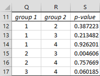
Figure 4 – Output from TUKEY function

Reference

Howell, D. C. (2010) Statistical methods for psychology (7^th ed.). Wadsworth, Cengage Learning.
https://labs.la.utexas.edu/gilden/files/2016/05/Statistics-Text.pdf

Tukey HSD (Honestly Significant Difference)