Building a Rasch Model

We show how to build a Rasch model via the following example. The approach described is based on the UCON method (i.e. unconditional maximum likelihood estimation using Newton’s Method).

Example

Example 1: Nine students (subjects) took a test consisting of the same 10 questions (items). Whether each student answered each of the questions correctly is shown in the data range A4:K13 of Figure 1. Note that for some reason question 1 was omitted from student A’s test (the missing data is shown in cell B5). Determine the ability ratings of each student and the difficulty of each question by using a Rasch model.

Figure 1 – Rasch model (initialization)

The values in range L5:L13 contain the percentage of questions each student answered correctly. E.g. cell L5 contains the worksheet formula =SUM(B5:K5)/COUNT(B5:K5). Similarly, range B14:K14 contains the percentage of students who answered each question correctly. E.g. cell C14 contains the formula =SUM(C5:C13)/COUNT(C5:C13) indicating that 88.9% of the students answered Q2 correctly.

First approximation for ability and difficulty

We now calculate the first approximation to the ability (range M5:M13) and difficulty (range B15:K15) values in the Rasch model. E.g. the ability of student A (cell M5) is 2.079, as calculated by the formula =LN(L5/(1-L5)), and the difficulty of question Q1 is -1.95 (cell B15), as calculated by the formula =LN((1-B14)/B14). Note that we didn’t use the formula =LN(B14/(1-B14)) in cell B15 since we want to force the easy questions to have a negative difficulty value and the hard questions to have a positive difficulty value.

Note that none of the values in L5:L13 or B14:K14 can be zero or one. This means that no subject can have all correct or all incorrect answers. Similarly, no item can be answered correctly by everyone or no one. E.g. if cell B13 contains 1 instead of 0 (and so everyone answers item 1 correctly), then the value of B14 would be 1 and so the value of =LN((1-B14)/B14) would be LN(0), which is undefined. Similarly, if cell J6 contains a 0 instead of 1 (and so no one answered item 9 correctly), then the value of J14 would be 0 and so the formula =LN((1-J14)/J14) would be undefined (division by zero).

This means that before starting the analysis you must remove any subject who answered all items correctly or incorrectly as well as any item that everyone or no one answered correctly. Note too that after removing such subjects/items, additional subjects/items might then qualify for elimination, and so this can be an iterative process.

The mean ability value (cell M14) is 0.419 as calculated by =AVERAGE(M5:M13). Similarly, the mean difficulty value (cell L15) is -.412. In order to make this mean come out to be zero, we need to adjust the difficulty values for each of the questions as shown in row 16. E.g. the formula in cell B16 is =B15-L$15. The mean of the adjusted difficulty value is now zero, as shown in cell L16.

Iteration

Expected values

So far, all that we have done is calculate the initial values for the ability and difficulty parameters. We now show how to improve these estimates using iteration. At each step in the iteration, we use the then-current estimate of the ability and difficulty parameters to calculate the expected values of the x_si using the formula

We then use these estimates to calculate improved estimates of the ability and difficulty parameters, and so on until no further improvement is necessary. In order to keep things simple, we won’t explain further why the described approach gives us the results we are looking for.

The expected values for P(x_si = 1 | β, δ) in iteration #1 are shown in Figure 2.

Figure 2 – Expected values (iteration #1)

E.g. cell B23 contains the formula =EXP($M5-B$16)/(1+EXP($M5-B$16)). Highlighting the range B23:K31 and pressing Ctrl-R and Ctrl-D will fill in all the other expected values. We will describe how to calculate the other values in the figure shortly.

Estimated variances

Figure 3 shows the estimated variances of these expected values. Here, we use the formula for the variance of the binomial distribution. Thus, the variance corresponding to cell B23 in Figure 2 is .026, as shown in cell O23 of Figure 3, as calculated by the formula =B23*(1-B23).

We next calculate the sum of the variances for each student (column Y), which will give an estimate of the variance of each ability parameter. E.g. cell Y23 contains the formula =SUM(O22:X22). The same approach is used to find the variances for the difficulty parameters (row 32).

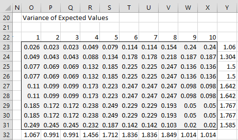
Figure 3 – Variance of expected values (iteration #1)

Residuals

We next calculate the residuals between our current estimates and the original data, as shown in Figure 4. Here, we place the formula =IF(ISNUMBER(B5),B5-B23,””) in cell AA23, highlight the range AA23:AJ31 and press Ctrl-R and Ctrl-D. We then calculate the sum of each of the rows in column AK and the sum of each of the columns in row 32.

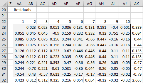
Figure 4 – Residuals (iteration #1)

Next, we calculate the sum of the squares of the row residuals in cell AK32 using the formula =SUMSQ(AK23:AK31). The goal of the iteration is to reduce this value to close to zero.

We now use the information in Figures 3 and 4 to arrive at improved estimates for the ability and difficulty parameters that are shown in Figure 2. E.g. the revised ability for student A is 2.872 (cell M23) as calculated by the formula =M5+AK23/Y23. The revised difficulty for item 1 is -1.93 (cell B33) as calculated by the formula =B16-AA32/O32. As we did previously, we need to reduce each of the difficulty parameters by -.07 (cell L33), which is the mean of the difficulty parameters in row 33 of Figure 2. The adjusted difficulty parameter values are shown in row 34.

Convergence

After performing 14 iterations, the sum of the squares of the row residuals (similar to the value in cell AK32 but after 14 iterations) will be reduced to less than .00001, which is close enough to zero for our purposes. At this point, the adjustments for the difficulty parameters are no longer necessary since the mean of the difficulty parameters is zero.

The expectation values after 14 iterations are displayed in Figure 5.

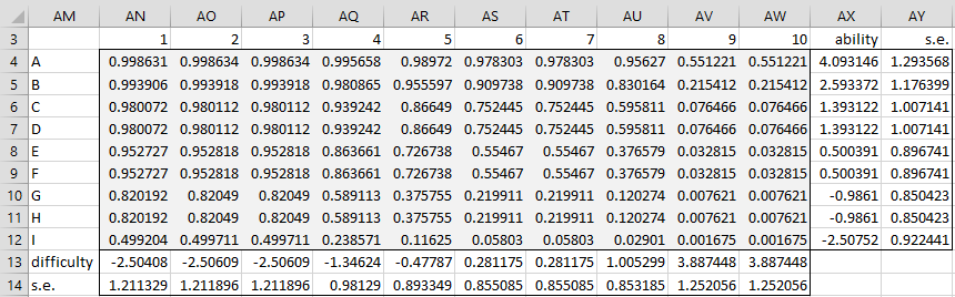
Figure 5 – Expectation values (after convergence)

This figure is similar to Figure 2, except that the standard errors of the ability and difficulty parameters are also displayed. The standard error of each ability and difficulty parameter is equal to the reciprocal of the square root of the variance calculated after 14 iterations. E.g. if we had only done 1 iteration, then the standard error of the ability of student A would be calculated by the formula =1/SQRT(Y23).

Fit

Figure 6 describes how well the resulting Rasch model fits the data.

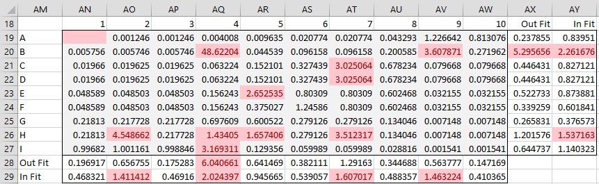
Figure 6 – Residuals (after convergence)

Each entry in range AN19:AW27 measures the fit of the model’s estimate of x_si and is equal to the squared residual divided by the variance. E.g. if we had terminated the model after one iteration, then we could calculate the value in cell AO19 via =IF(ISNUMBER(C5),(C5-AO4)^2/P23,””) and similarly for the other cells in the range. The formula that is actually used is the same except that cell P23 is replaced by the variance calculated for student A on Q2 after 14 iterations (not 1).

All fit statistics that exceed 1.3 are highlighted. These represent outliers, i.e. expected x_si values from the model that don’t fit the data very well (although you can ignore highlighting corresponding to missing data values such as in cell AN19).

Infit and Outfit

Figure 6 also includes two statistics, infit (information-weighted fit) and outfit (outlier-sensitive fit), that measure the fit of the ability and difficulty parameters. The outfit values are simply the mean of the corresponding residuals. E.g. the outfit for the ability of student A is .238 (cell AX19), as calculated via =AVERAGE(AN19:AW19), which is well within the 1.3 target. The outfit value for student B at 5.30 is an outlier, and so is highlighted.

The calculation of the infit statistic is a little more complicated. Again, if we had terminated the model after one iteration the formula for the infit statistic for item Q1 could be calculated by the worksheet formula =SUMSQ(AA23:AA31)/SUM(O23:O31). As before, instead of using the values from iteration #1, we actually use those from iteration #14.

Any infit or outfit values that exceed 1.3 are highlighted and may indicate a sub-optimal fit and are flagged for investigation as to a possible cause.

Possible reasons for an ability misfit are that the subject is guessing or the subject is different from the target population. Misfit values are to be expected with small samples. One approach to investigating a misfit is to set misfit items for this subject to missing to see whether this resolves the problem, in which case perhaps the subject didn’t understand the question. Another approach is to remove the subject from the data set and rerun the analysis to see what happens.

Possible reasons for an item misfit are that the question is confusing or not worded well. Perhaps the item is not testing the intended skill. One approach to dealing with an item misfit is to remove the item from the data set and repeat the analysis.

Conditional formatting

The highlighting shown in Figure 6 can be accomplished by using conditional formatting.  This is done by highlighting range AN19:AW29 and selecting Home > Styles|Conditional Formatting. On the dropdown menu that appears select the Highlight Cell Rules and then Greater Than options. In the dialog box that appears insert 1.3 and press the OK button.

You need to repeat the same process for the range AX19:AY27. You could have performed conditional highlighting on the complete range AN19:AY29, but then the lower right blank portion of the range would also be highlighted.

Examples Workbook

Click here to download the Excel workbook with the examples described on this webpage.

References

Moultan, M. H. (2003) Rasch estimation demonstration spreadsheet
https://www.rasch.org/moulton.htm

Wright, B. D. and Stone, M. H. (1979) Best test design. MESA Press: Chicago, IL
https://research.acer.edu.au/measurement/1/

Wright, B. D. and Masters, J. N. (1982) Rating scale analysis. MESA Press: Chicago, IL
https://research.acer.edu.au/measurement/2/

Boone, W. J. (2016) Rasch analysis for instrument development: why, when, and how?
https://www.ncbi.nlm.nih.gov/pmc/articles/PMC5132390/pdf/rm4.pdf

Boone, W. J. and Noltemeyer, A. (2017) Rasch analysis: A primer for school psychology researchers and practitioners. Cogent Education
https://edisciplinas.usp.br/mod/resource/view.php?id=3333001

Furr, M. and Bacharach, V. R. (2007) Psychometrics: an introduction; Chapter 13: Item response theory and Rasch models. Sage Publishing
https://in.sagepub.com/sites/default/files/upm-binaries/18480_Chapter_13.pdf

Wright, B. and Stone, M. (1999) Measurement essentials, 2^nd ed.
https://www.rasch.org/measess/