Basic Concepts
In the Holt-Winters Method (aka Triple Exponential Smoothing), we add a seasonal component to Holt’s Linear Trend Model. We explore two such models: the multiplicative seasonality model and the additive seasonality model. We consider the first of these models on this webpage. See Holt-Winters Additive Model for the second model.
Let c be the length of a seasonal cycle. Thus c = 12 for months in a year, c = 7 for days in a week, and c = 4 for quarters in a year. The model takes the following recursive form for all i > c
![]()
![]()
![]()
where 0 ≤ α ≤ 1, 0 ≤ β ≤ 1 and 0 ≤ γ ≤ 1.
The ui values represent the baseline, the vi values represent the trend (i.e. slope) and the si values represent the seasonality component. In the multiplicative model, for any consecutive c periods of time, the sum of the si values is approximately equal to c (at least for reasonable values of α, β, γ).
The predictions for the data elements yi can be expressed by
![]()
For forecasts at future times, we use the form
![]() where h′ =INT((h–1)/c)+1.
where h′ =INT((h–1)/c)+1.
Alternative Forms
We can also use the following alternative version of the seasonality term:
![]()
Based on this version of the seasonality term, we have the following alternative form of the recursive equations:
![]()
![]()
![]()
![]()
The initial values for the model, i.e. where 1 ≤ i ≤ c, are
![]()
Alternatively, we can set the initial trend value by using the average slope for the first two years, namely:
![]()
Note that if γ = 0, then the Holt-Winters model is equivalent to Holt’s Linear Trend Model, and if β = 0 and γ = 0, then the Holt-Winters model is equivalent to the Simple Exponential Smoothing Model.
Examples
Example 1: Calculate the forecasted values of the time series shown in range C4:C19 of Figure 1 using the Holt-Winter method with α = .5, β = .5 and γ = .5.
The result is shown in Figure 1. First, we calculate s1, s2, s3, s4, where c = 4, as shown in range F4:F7. We do this by inserting the formula =C4/AVERAGE(C$4:C$7) in cell F4, highlighting the range F4:F7, and pressing Ctrl-D.
Next, we calculate uc and vc by placing the formula =C7/F7 in cell D7 and the value 0 in cell E7.
We now insert the formula =C$22*C8/F4+(1-C$22)*(D7+E7) in cell D8, the formula =D$22*(D8-D7)+(1-D$22)*E7 in cell E8, =E$22*(C8/D8)+(1-E$22)*F4 in cell F8 and the formula =(D7+E7)*F4 in cell G8, and then highlight the range D8:F19 and press Ctrl-D.

Figure 1 – Holt-Winters Multiplicative Method
Example 2: Forecast the y values for 2014 from Example 1 (i.e. the next 4 quarters).
The result is shown in Figure 2. The values through 2013 are copied from Figure 1. The forecasted value for Q1 of 2014 is 36.87209 (cell N20), as calculated by the following formula with reference to cells in Figure 1.
=(D$19+(L20-L$19)*E$19)*F16
The other three forecasted values are calculated by highlighting the range N20:N23 and pressing Ctrl-D.
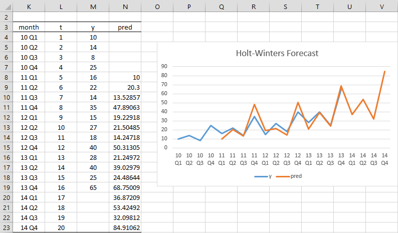
Figure 2 – Holt-Winters’ Multiplicative Forecast
Optimization
As we have done in Example 2 of Holt’s Linear Trend, we can use Solver to determine which values of alpha, beta, and gamma yield the best Holt-Winters fit for the data in Example 1.
The optimization approach using Excel’s Solver, however, is susceptible to finding a local minimum instead of a global minimum. For this reason, the optimized values for alpha, beta, and gamma are sensitive to the initial values used. You can have Solver try out different initial values to find parameter values that reduce the value of MAE.
To do this, select Data > Analysis|Solver and press the Options button on the Solver dialog box. The Solver dialog box automatically contains the values collected by the Basic Forecasting data analysis tool. Now, choose the Multistart option from the GRG Nonlinear tab of the Options dialog box. Solver will now run multiple times using different starting values, picking the values that produce the best outcome. The cost of this option is slower run times.
In Real Statistics Forecasting Tools, we use a slightly different approach to improve on the optimization approach. This follows along the lines described in Holt’s Trend Confidence Interval.
Examples Workbook
Click here to download the Excel workbook with the examples described on this webpage.
Reference
Hyndman, R. J., and Athanasopoulos, G. (2021) Holt-Winters’ seasonal method. Forecasting: principals and practice, 3rd Ed.
https://otexts.com/fpp3/holt-winters.html
Hi Charles,
Considering the fact that seasonality in a data set can be less obvious/visible in some cases, would it not be advisable to use HWM then instead of going straight with HLT ? The optimisation would set the gamma component to zero or close to it when no seasonality is detected, making the results equal to HWM in this case. Or is this approach not correct ?
Hi Dirk,
I agree with you. I can’t think of any drawback to your approach, although there may be.
Charles
Hi Charles,
1. I have a data series of 240 EOM stock prices. I have converted this into annualised returns using the LN function which gives me in essence 240 years of return data now. Would it make sense to run a forecasting model HWA or HWM or even Arima over annualised return data instead of raw price data ? I presume the data would be stationary and no additional detrending would be necessary. Would there be any advantages in doing so ? Your opinion is much appreciated.
2. Other than this, a great stats website you have put together. It’s been a help in many ways already. Any other means that Paypal for a donation ?
Cheers and keep up the good work,
Dirk
Belgium
Hello Dirk,
1. There are many approaches for forecasting, including HWA, HWM, and Arima. I assume that your data has a trend and seasonality (otherwise you probably wouldn’t have included HWA and HWM).
Why do you presume that your data is stationary? If it is, then probably detrending wouldn’t be necessary.
2. Thank you very much for your kind remarks and support.
The only approach that I have set up for donations is Paypal.
Charles
Charles,
Thanks for your reply.
The data indeed has a trend but no seasonality is present.
Stationarity of the data would still have to be verified. I presume annualising this raw data over 12 periods with the LN function would make it stationary (or close to it). I’ll have a look using the ADF test just to make sure. If I want to use Arima it would have to be stationary, HWA and HWM does not really require stationarity (I presume).
Dirk,
If the data doesn’t have seasonality you could use Holt’s Linear Trend instead of HWA or HWM.
Charles
Charles,
Yes indeed, HLT would be better as you say. Meanwhile I found out that annualising the price data with the LN function does not result in stationarity of the series. Differencing once does the trick. Then Arima and HWA produce adequate results, however I think forecasting would work better with the raw price data, going by the metrics.
Prof. Zaiontz, this article (and the Additive Model’s article) constrains “where 0 < α ≤ 1". Did you mean to specify 0 ≤ α ≤ 1 (greater than OR equal to 0)? As required by your Resource Pack, should I add 'gamma ≥ 1 – alpha' as a constraint in Solver (when not using your Resource Pack)? Thanks.
Correction: As required by your Resource Pack, should I add ‘gamma ≤ 1 – alpha’ as a constraint in Solver (when not using your Resource Pack)?
Jim,
In an earlier version of this webpage, I required that gamma ≤ 1 – alpha. I have since replaced gamma by gamma* as defined at
https://otexts.com/fpp3/holt-winters.html
although I still call it gamma (without the star). In this case, the requirement is 0 <= gamma <= 1. Charles
Hi Jim,
I believe that 0 ≤ α ≤ 1 is correct. I probably saw it in another resource as 0 < α ≤ 1, but I believe that the first inequality is correct. Charles
Dear Charles,
Thanks for this wonderful work!
I have observed people asking about forecasting further out than c. I am using my company computer and it does not allow me to download Real Statistics Resource Pack. And therefore I have no idea how you approached forecasting further out than c in your program. Can you please elaborate further?
I don’t know if it makes sense, but my approach was the following:
* For the first point after c periods, we will be needing the seasonality term of the first forecasted period.
* The seasonality term requires a Level estimation. The Level estimation requires realized values, however, given that we are now in the forecasted future, I have used the forecasted value instead of the realized value in the equation, making it become: Alpha x (Forecast / Seasonality Term of c periods ago) + (1 – Alpha) x (Level of 1 period ago + Trend of 1 period ago)
* Coming back to the seasonality term; it is normally calculated using the realized values, however, given that we are now in the forecasted future, I have used the forecasted value instead of the realized value in the equation, making it become: Gamma x (Forecast / Level) + (1- Gamma) x (Seasonality Term of c periods ago)
* Now I can use the seasonality term of the first forecasted value, for the calculation of the forecast value for the period, c+1 periods after the final realized data.
Dear Atlas,
The forecast values after c are calculated in the same manner as those prior to c. In fact, the following webpage gives an example where c = 4 yet 6 periods are forecasted.
https://www.real-statistics.com/time-series-analysis/basic-time-series-forecasting/real-statistics-forecasting-tools/
I have also added a link to the spreadsheet that shows how the forecast was calculated.
Charles
Hi Charles,
I was wondering how you would forecast past the seasonal level? i.e. forecasting monthly sales, I understand how to forecast 12 months into the future by using the seasonal calculations, but how would you forecast 18 months as you ‘run out’ of seasonal data to use as it only covers 12 months into the future
Thanks, Kade
my only thought so far would be to use the forecasts I have already made (the 12 months out of sample forecasts) to calculate the 18 months out of sample forecasts by using that data as if it has already occurred even though it is only forecasted
thanks, Kade
Hello Kade,
See my previous response.
Charles
Hi Kade,
I don’t see why you couldn’t forecast more than 12 months into the future. I suggest that you try it out. See, for example, the following webpage
https://www.real-statistics.com/time-series-analysis/basic-time-series-forecasting/real-statistics-forecasting-tools/
The example on this webpage uses quarterly seasonality, but forecasts 6 quarters into the future and not just 4 quarters into the future.
Charles
Hi charles, was wondering for the real stat tool, what is the lag option referring?
Just seen when u hover over says for moving average. Thought it was affecting the holts winter’s method as well.
Hello Exer,
Sorry, but I don’t understand what you are referring to. I don’t see anything unusual when I hover over Moving Average.
Charles
Hello Exer,
It is only used with the Simple Moving Average option. See
https://www.real-statistics.com/time-series-analysis/basic-time-series-forecasting/real-statistics-forecasting-tools/
Charles
Hai charles thanks for article, sorry but i don’t understand why value Vi is zero at E7. Can you help me for that and how derivation and proof formula of holt winters exponential smoothing?
Ahyo,
In general, v_i+1 depends on v_i. E7 is arbitrarily set to zero to initiate the v variable.
The formulas define Holt-Winters method. As a result, there isn’t a proof. See the reference at the end of the web page for more details.
Charles
Thanks charles, I’ll look at the web reference later. I am really very confused because my lecturer asked me how to derivation the formula, or prove the formula for Holt Winters exponential smoothing. like how the formula levels, seasonality and trend started. does it come from arima etc, like that
Hello Ahyo,
See the following
https://stats.stackexchange.com/questions/229384/use-holt-winters-or-arima#:~:text=R's%20arima%20%2C%20for%20example%2C%20uses,doesn't%20tell%20you%20much.
https://www.scirp.org/journal/paperinformation.aspx?paperid=108951
Charles
Hello Charles Sir,
I am doing a research project and want to use the Holt Winters Method. and I am looking for an excel sheet as an example with the Formulae (like the one whose image you have pasted in the article).
Is it possible to send me the xcel sheet which will help me understand this better.
I shall be highly grateful to you
Best Regards
You can download the Excel sheet for any of the examples found on the Real Statistics website. Please go to
https://www.real-statistics.com/free-download/real-statistics-examples-workbook/
Charles
In the first formula, you have
> where 0 < α ≤ 1, 0 ≤ β ≤ 1 and 0 ≤ γ ≤ 1–α.
. Is that correct? For the form you're using, isn't 0 ≤ γ ≤ 1 ?
See https://otexts.com/fpp3/holt-winters.html
Hell Marco,
Yes, you are correct. I have corrected this on the website (and made a similar change for the additive version of Holt-Winters).
Thank you very much for your help and I apologize for my delayed response to your comment.
Charles
I cannot thank you enough for creating this explanation and downloadable examples.
I had been relying on the wikipage (“Exponential Smoothing”), which leaves much to the imagination — and some of which seems incorrect.
As I work through your details (WIP), I hope it is okay if I make note of some apparent inconsistencies (subject to your review) from time to time. For example….
—–
1. You write:
(a) “In the multiplicative model, for any consecutive c periods of time, the sum of the si values is approximately equal to 1“.
and
(b) For the additive method: “The sum of the seasonality components for c consecutive periods of time is approximately c (not 1 as in the multiplicative model).“
Errata: It appears to be c for multiplicative, as well as for additive.
In your “Holt-Winter” worksheet (multiplicative), the average sum of “c” consecutive s[i] values is 4 (c), not 1, for the example model where c=4 and alpha=beta=gamma=0.5.
In fact, the average sum rounds to 4 (c) in 89% of 1000 trials with random alpha, beta and gamma (gamma <= 1-alpha).
And I have not seen 1. The min average sum rounds to 4.
—–
2. OTOH, the max average sum of s[i] values rounds to 6.70 when alpha=0.003092692913089, beta=0.718335362652918 and gamma=0.934268804623004 in the "Holt-Winter" worksheet (multiplicative).
And the relative sd is large, with min sum of s[i]=4.39 and max sum of s[i]=10.2.
So, I wonder if it would be helpful to add limits on the expected average sum of s[i] values as additional criteria for finding a "good" set of alpha, beta and gamma. For example, C22:E22=3.5 for c=4.
And I wonder if it would be helpful to add similar limits on the min and max sum of s[i] values, as well. For example, both must be between 3.5 and 4.5 for c=4.
Hi Joe,
Sorry for the late response.
Yes, you are correct. I have modified the webpage to reflect this.
Thank you very much for identifying this error and for improving the accuracy and useability of the website.
Charles
Dear Charles,
this site is really helpful.
Great explanation in this webpage and the Add-Ins for Excel.
Is it possible to find another Add-Ins for Excel that includes Holt Winters with application of Nelder Mead method for coefficients optimization?
Dear Riccardo,
That is indeed a good idea since Solver doesn’t always find the optimum coefficients.
I will consider using Nelder Mead, although I have been thinking about using a different approach.
Charles
Dear Charles, thanks you for the answer and for all in your wonderful and amazing site. Riccardo
Dear Charles,
thank you very much for this webpage and the Add-Ins for Excel. I am trying them out at the moment and I have a few questions:
– Why is it necessary that Alpha + Gamma is smaller than or equal to 1? And why is it – using Solver – mostly exactly equal to 1? I have read the Wikipedia Page about Exponential Smoothing and there is no such condition.
– How is the best way to choose the parameters yourself? Is it always best to minimize some kind of error or are there other methods? Do you know with which method they are chosen in the excel forecast function forecast.ets? Or is there some possibility to choose it yourself?
Thank you very much in advance!
Janne
Dear Janne,
1. Regarding the restriction about alpha and gamma, see
https://otexts.com/fpp2/holt-winters.html
2. I used Solver to minimize MSE, MAE or RMSE, as explained at
https://www.real-statistics.com/time-series-analysis/basic-time-series-forecasting/holt-linear-trend/
3. I believe that Excel uses Holt-Winters’ Additive model (not the multiplicative version). See
https://www.real-statistics.com/time-series-analysis/basic-time-series-forecasting/excel-2016-forecasting-functions/
https://www.real-statistics.com/time-series-analysis/basic-time-series-forecasting/holt-winters-additive/
Charles
Dear Charles,
thank you very much for your fast answer.
I have another problem that came up with the Excel add-ins: Every time I do a forecast with it, the tab “Add-Ins” closes and to be able to do another forecast, I have to close my document, I have to remove the check at “Xrealstats” (in Developer tools -> Excel add-ins), then wait, check “Xrealstats” again, wait again and the tab “Add-Ins” with “Real Statistics” reappears and I can do another forecast. Do you know this problem? Do you have any ideas how to solve it?
Concerning the choice of Alpha, Beta and Gamma: Do you know any other methods than the one you use?
Concerning the Excel forecast function forecast.ets: Yes, it uses the additive method. But I would really like to know with which algorithm/method Excel chooses the parameters. Until now I couldn’t find it out.
Thank you very much in advance!
Best regards,
Janne
Hello Janne,
1. Regarding the problem of the AddIns ribbon, see
https://www.real-statistics.com/appendix/faqs/disappearing-addins-ribbon/
2. Here is another approach for estimating these parameters (essentially a grid search).
https://www.researchgate.net/publication/336564436_Determination_of_Optimal_Smoothing_Constants_for_Holt_-Winter's_Multiplicative_Method
3. I don’t know how they determine the values of the parameters. I will try to find out, but I think I tried in the past without success.
Charles
Dear Charles,
thank you very much again for your fast answer!
Concerning the Add-Ins ribbon, I haven’t found a solution yet, but I will keep on trying. (Ctrl-m doesn’t seem to work for me…)
Concerning the values of the parameters for the Excel forecast function forecast.ets, I already tryed to find out as well, without success. I just thought you might perhaps know.
Best regards,
Janne
Dear Charles,
First of all, thank you very much for your article, its truly great and easy to understand.
I have tried to use the learned on own dataset but faced some issues when forecasting, namely forecast quickly tends to negative values instead of following the normal trend. It is a dataset with 24h periodicity with Gaussian like distribution / day with peaks between 10h-14h (traffic statistics).
I have 1390 historical rows (~58 days, 2 rows are missing actually) where last known ‘u’ and ‘v’ values calculated from historical data are:
u_1390 = 1.07546
v_1390 = -0.16529
As ‘s’ is always positive, pred = (u_1390 + (t – 1390) * v_1390) * s_1368 equation quickly leads to a decreasing trend after t = 1391, 1392, etc. where increasing periods do not “come back” at all.
Used formulas are correct, I have checked with your data and everything fits your results. Prediction on historical data is also OK with my dataset but forecast fails.
Unfortunately I cannot upload file or screenshot but I would be happy to send you by e-mail.
Could you please check what could be a problem? Is it possible that HW method is not applicable for such dataset?
Thank you very much in advance,
All the best,
Tamas
Tamas,
Yes, please send me an Excel file with your data and forecast results.
Charles
Hi Charles,
What is the logic behind forcing α and β to be less than 1 ?
In most forecasting models I have seen, this is not really necessary.
Thanks
Murad
Murad,
These are weights. Think of alpha as dividing 1 into alpha and 1-alpha. Similarly for beta.
You said that in most forecasting models these restrictions are not necessary. Can you give me a reference to one such model or give me an example where the values of alpha and beta are not between 0 and 1?
Charles
Thanks for the article.
What does INT mean here?
h′ =INT((h–1)/c)+1.
Tom,
INT(x) is the largest integer smaller than x. Thus, INT(3) = 3, INT(3.7) = 3 and INT(-3.7) = -4.
Charles
Thank you so much for your help!
Dear Charles, thank you very much for your article.
I would like to ask kindly a question: I have data which shows clearly a negative trend (T-Test confirms) . I deseasonalized the data to get the initial level and trend estimates via a trendline on the deseasonalized series. The initial values for the trend (-0.7) is negative. Now using Solver in Excel, yields for the trend smoothing parameter simply 0 because I set the constraint that only values between 0 and 1 are allowed. If data shows a negative trend is it correct if the solver is simply puts the trend smoothing parameter to 0 and the model continues to calculate with the initial trend value (-0.7) ?
Best Regards,
Nic
Hello Nic,
I am a bit confused. Why did you constrain the trend to values between 0 and 1 when you know that the trend is negative?
Charles
Hi Charles,
Thank you for your reply, it is very much appreciated. Initially I thought the data would yield a positive trend, not negative. Hence I did not adjust the constraints of smoothing parameters. If the data shows a negative trend, I can/should lower the solver constraint regarding the trend smoothing parameter to -1?
Best Regards,
Nicolas
Hi Charles,
Do you think that optimizing the parameter value (using solver) would result in over-fitting ?
Murad,
I know that Solver doesn’t always find the global optimum parameter value and can instead find a local optimum value.
I don’t know whether it results in overfitting.
Charles
Hello Mr Charles, thanks for this great explanation. However when I tried to forecast for the next quarters on my own, if observed that the (Si+h-ch’) should be 14 instead of 13 used on this page because I got the value of (h’) to be 1. I hope I am not mistaken.
Thanks in advance!
Hello,
Which cell in the spreadsheet are you referring to? What is the value of i?
Charles
Hello,
Can someone please help me solve Holt’s model by hand using a multiplicative trend or even tell me a page in which I can find examples because I’m having it hard to find a page which explains these examples without excel, this are the information I have:
Assume you are working with monthly data, with December being month
12, January being month 13 etc. Suppose L12 = 80 and T12 = 1.2 and you
observe Y13 = 90. Determine the forecast for Y15, assuming α = 0.3 and
β = 0.7 using a multiplicative trend.
Thank you in advance.
Hello Didi,
This is explained on this webpage. What items are not clear?
Charles
In excel how would I add a damping effect (phi)
Jeff,
The references for this topic tell how to add the damping effect, but I haven’t yet added this to the website or Excel software.
Charles
Charles
Can you point me to the reference?
Never mind I found it.
Hi Charles,
Can you make forecasts beyond one season using this method?
Neeta
Neeta,
Yes, you can.
Charles
How?
Sorry but I don’t understand what you are referring to.
Charles
Dear Sir,
Your explanations are so clear. I understand there are various methods to attain the starting values in HW. Pls share whose method you have used here. does the initial values are deseasonalised? Thank You
Hello Asha,
There are many ways of setting the initial values. Two such approaches are described on this webpage just above Example 1.
Charles
Hey Charles,
thanks for putting this site together!
Is there a way to set a “floor” with Holt Winters? For instance, if sales trends have been negative for a long time the forecast continues to be negative and predicting a monthly forecast beyond 4-6 months starts to produce unrealistic (less than zero) results. Is there a way to set a minimum threshold that prediction cannot go below?
Thanks
Hello Brian,
If you use Solver, then you can set a floor.
Charles
Hi Charles,
I have followed your method and the final alpha, beta and gamma values provided to me by the Solver are dependent on the initial values alpha, beta and gamma values I input.
Is that supposed to happen?
For example: If I have 0.5 as my initial alpha, beta and gamma values, Solver gives me alpha = 0.46, beta = 0.5 and gamma = 0.54.
Whereas, If I have 0.6 as my initial alpha, beta and gamma values, Solver gives me alpha = 0.48, beta = 0.6 and gamma = 0.48.
P.S. I have set my objective in the Solver to minimize MAE
Hello Yash,
In general, it is possible that the results will depend on the initial parameter values. Whether or not this is so for this situation, I can’t say. If you send me an Excel file with your data, I will give you a more precise answer.
Charles
Note in this excellent excel implementation the seasonality includes the term y(i)/u(i), rather than y(i)/(u(i-1)+v(i-1)) as shown in https://otexts.com/fpp2/holt-winters.html (1)
A hasty check suggests this isn’t critical. But when implementing Holt-Winters’ damped method (1) then I *think* the original equation is easier to work with.
(1) Hyndman, R.J., & Athanasopoulos, G. (2018) Forecasting: principles and practice, 2nd edition, OTexts: Melbourne, Australia. OTexts.com/fpp2. Accessed on 23 Jun 2019
Hello Vahid,
Yes, I am familiar with Hyndman’s OTexts. I haven’t implemented the damped method yet, but I will eventually add it.
Charles
Hi Charles,
Hyndman appears to reference this point: “In many books, the seasonal equation…is slightly different from these, but I prefer the version above because it makes it easier to write the system in state space form. In practice, the modified form makes very little difference to the forecasts.”
https://robjhyndman.com/hyndsight/hw-initialization/
So I believe the equations you used are the original form which ‘m sure you already knew. I’m just happy knowing that my loose end was conveniently resolved.
Hello,
Do you know if there is a specific scale of judgement of forecast accuracy for the Error measures you used? In this case MAE and MSE. How can you tell if your obtained error is adequate, too small or too big. (for both error measures)
Thank you in advance for answering.
Hello Clark,
There is no simple answer to this question. The smaller MSE (or MAE) the better. Thus if you have two models, one with MSE of 10 and the other MSE of 9, then all other things being equal, you prefer the one that has MSE equal to 9.
Ideally you should build your model with part of the data and then test to see how good your model does with the rest of the data (where you already know the correct forecast values (namely the actual values). This is called cross validation.
Charles
Hello,
Is your version of Winter-Holt’s the additive or multiplicative method?
Hello Tamika,
Additive method.
Charles
Thanks for your response. May I ask why you chose the additive over the multiplicative? I also read that there are various ways to initialize the Winter Holt’s method. Can you explain the pros and cons of each type?
Hello Tamika,
I looked into this further and see that the info I gave you previously was wrong. I seem to be using a multiplicative model, but it seems to be a little different from the standard model. As a result, I plan to investigate this further and if necessary change it to the standard model in the next release. I will also include both the additive and multiplicative models. I hope to have this available in the next few days.
Thanks for raising this issue.
Charles
Tamika,
I have now looked into this further, and found that the approach I used was the standard approach, although I plan to change the initial values in the next release. I will also correct the forecast values for the data, which will change the optimized values. Finally, I will also add the additive version.
Charles
Thank you Charles for this information. The wealth of knowledge that you are providing is appreciated. May I ask if your Real Statistics add-in can be used for Data Mining?
Tamika,
The Real Statistics add-in can be used for data mining, e.g. cluster analysis and regression, but other capabilities are not yet covered.
Charles
HEY,
i have some questions for how to choose the period , here is my question
1) if i have 1 year of daily data means it is 365 entries (it’s not a leap year) So period is 364
now
2) if it is leap year means 366 entries , now what is the period ?? because 365 gives a wrong forecast
3)why exponential smoothing is not taking 364 while total num of data is 366?
4) ExponentialSmoothing(dataframe ,seasonal_periods=period ,trend=trend,damped=True , seasonal=seasonal) this syntax i am using
5) but if we have two year of data like (365+366) or (365+365) then period 364 gives a expected output
help will be appreciated
thanks
Hello,
1. The period is 365, but unless you are going to look at trends from a specific day (e.g. Jan 4) or days from year to year, there is no point in taking seasonality into account. In this case, you might as well use the Holt’s Linear Trend model.
2. 366, but see response to #1.
3. I don’t understand what you mean by “…is not taking 364”.
4. I don’t know which software package you are referring to.
Charles
Goedemiddag,
Ik heb een vraag:
Ik werk in een productie organisatie en wil de forecast optimaliseren.
Mijn vraag/stelling is als volgt:
Huidige week = 4. (maandag!) De afzet van week 4 is dan niet niet totaal bekend.
Plannen voor = week 5
Afzet = week 6.
Hoe kan ik tijdig de forecast aanpassen voor week 5(productieweek) o.b.v. historische data (Moving Avarage).
En hoe kan ik deze trend doortrekken naar week 6,7,8,9,10 enz. als ik nog niet op de hoogte ben van de werkelijke afzet in deze weken ?
Hello Daniel,
These types of forecasting issues are not so easy to solve. These sorts of issues are more art than science and are not easy to answer quickly.
I suggest that you try different forecasting models holding out some of the data so that you can evaluate the accuracy of each model based on the real data that you held out.
Charles
Hi Charles
Great work!
I just wonder why Excel 2016’s ETS (exponential triple smoothing) forecast function
=FORECAST.ETS provides another result than yours Holt-Winters forecast.
Thanks.
Hi Alex,
Can you send me an Excel file with your data and the results you obtained from the FORECAST.ETS function? I will try to figure out why you are getting different results. There a number of different implementations of ETS/Holt-Winters and so Real Statistics may be using a version different from the one chosen by Microsoft.
Charles
Excel ETS can result in a very spiky FC fit at times for no apparent reason. Holt-Winters (add) performs better in my opinion.
I stumbled upon this page whilst researching how SAP APO Statistical Forecast models were generating their Basic, Seasonal, Trend values. After reading so many articles that talk theory only this is a fantastic practical example which actually clearly demonstrates the calculations. Thanks so much for putting this together.
Cook,
Glad that the website was helpful to you. I try my best.
Charles
Hey Charles
Thanks a million for this. Please can you specify how do you calculate the rest of seasonal indices after 10 Q4?
Fahad,
Suppose you want to forecast one more year (11 Q1, 11 Q2, 11 Q3, 11 Q4). One approach is to copy the range L23:N23 into the range L24:N24. L24 should contain the value 20 and N24 should contain the formula =(D$19+(L24-L$19)*E$19)*F20. Now replace F20 by F16 in this formula (the latest estimate for Q1). Next highlight the range L24:N27 and press Ctrl-D.
Charles
can alpha, beta or gamma take negative values?
No, they cannot be negative.
Charles
Hi Charles,
Could you please advise the logic behind γ factor should be less than 1–α (aka γ < 1–α) ?
My understanding γ value can be in the range of 0 – 1.00.
Thank you in advance!
Yozie,
See https://www.otexts.org/fpp/7/5
Charles
This site is really helpful and the example is a godsend!
One question. Shouldn’t, in equation 1, the variable w sub(i-c) in the equation for u sub i,
be the variable s sub (i-c)?
Also,
shouldn’t in equation 3 be S sub i instead of w sub i?
Peter
Peter,
You are absolutely correct. Thank you very much for identifying this error. At one time I used the symbol w instead of s, but forgot to change it in all places. I have now corrected the error.
I appreciate your help in improving the website and making it easier for people to understand what is going on.
Charles
Hi Charles,
Great explanation. .. as I followed your example, I noticed the moving sum of the new calculated s over C periods is no longer equal to C or averaging to 1. How important is it to normalize C as we use Holt Winter model?
I reworked the example using normalized s figures, and the MSE improved to 34.53; however, MAPE deteriorated from 17.91% to 18.22%.
I appreciate your view on this.
Thanks.
Ayman,
This true for the first year since that is how the values are initiated. After the first year it is not necessary for any consecutive 4 quarter period to average to 1.0. In fact it would be impossible unless all the quarter 1 values are the same, and similarly for Q2, Q3 and Q4.
Charles
Awesome, thank you!
However I do have a question, and I cannot find the answer in any of the tutorials.
It’s a simple question probably everyone will encounter:
How do I forecast for more than one season?
Assume that I’m using the Additive model, my daily data shows a strong weekly recurrence, usually when we predict for the next season(week) we fix the level and trend components of the last day of previous week and use the seasonal component of the same weekday of last week. But what shall I do if I want to forecast more than 1 week?
Thank you!
Markus,
You can forecast as many seasons as you like using Holt-Winters. If you are using the Real Statistics data analysis tool just make the # of Forecasts value as large as you need (e.g. enter 14 for 2 weeks).
Charles
Hi Charles thanks for the reply!
Dear Charles,
I replicated your model, then applied “=FORECAST.ETS” function (as well as “Forecast Sheet” in the Data Tab, which uses the same “ETS AAA” algorithm). ETS AAA Excel algorithm is stated to implement Holt-Winters method.
The first issue is that ETS AAA choses alpha, beta and gamma, which are 0.251 / 0.001 / 0.001 respectively for your example data. These Excel algorythm values of α, β, γ are even worse than your initial 0.5/ 0.5 / 0.5 in terms of MSE (Excel figures worsened the error by around 8 points).
The second issue is that even if we accept 0.251 / 0.001 / 0.001 for α, β, γ, the predictions are different:
* in your model the predictions are as follows (decimals are shortened but not rounded):
24,7 for period #17
34,6 for period #18
19,8 for period #19
61,9 for period #20
* Excel’s ETS AAA (claimed to be Holt-Winters) algorithm predicts:
38,5 for period #17
47,3 for period #18
41,2 for period #19
60,3 for period #20
To sum up, my ultimate concerns are rather simple: “Can we securely use Excel’s “=FORECAST.ETS” function, believing it is backed by established Holt-Winters method? Otherwise, should we avoid using Excel’s ETS AAA, for we don’t understand the calculations behind this ‘black box’ algorythm?”
Thank you
Dmitry,
I honestly don’t understand the Excel calculations either. I would imagine that they make sense, but I need to find some reference that explains the calculations. I know that they don’t agree with the values produced by the Real Statistics software. I will try to find something that explains what is going on and get back to you.
Charles
Dmitry,
Apparently, others share your concern about Excel’s FORECAST.ETS function. See the following:
https://social.technet.microsoft.com/Forums/ie/en-US/b29d4216-3882-4883-86de-4b16157f491f/calculation-transparency-behind-forecastets-function?forum=excel
Charles
Charles,
Thank you for your opinion and the link. I haven’t seen the later.
Dmitry
FORECAST.ETS() appears to assume additive seasonality. This becomes clear when forecasting well beyond the original data set and noting the seasonal component does not grow with trend.
This site is a fantastic resource!
Great explanation but is it possible to use Winter’s model to forecast farther out than c observations (4 in this case)? What ways are their to forecast say for 2015 or 2016 in this example?
Mike,
Yes, you can forecast further out than c. Keep in mind, the further out you go the less accurate the forecast will be. See the following webpage regarding how to specify longer forecasting periods using Real Statistics:
Forecasting Tools
Charles
The link you have mentioned does not explain how to forecast further out than c. Kindly show how can we forecast for 2015 or 2016 using excel formula only.
Namita,
If you have Excel 2016 and want to use only pure Excel formulas, then see the following webpage:
https://real-statistics.com/time-series-analysis/basic-time-series-forecasting/excel-2016-forecasting-functions/
Charles
very nice, just need a clarification, for prediction the formula is =(D$18+(L20-L$19)*E$18)*F16, why D$18 and E$18 NOT D$19 E$19 as, it predicts the value of 20.
Debadrita Panda,
You are correct. Thank you very much for identifying this error. I have now corrected the error on the referenced webpage.
I really appreciate your help in improving the Real Statistics website.
Charles
Hi Charles,
Thanks for the help.
If the time series data has y=0 as some entry the calculation for S and u, v start giving DIV#0 error. If i replace 0 with a very small number like 0.001 the value for initial S goes very low and value of u,v gets multiplied by same factor and the forecast has huge errors.
Sample Data : YEAR Month mm
2012 Jan 16.7
2012 Feb 0
2012 Mar 0
2012 Apr 8.2
2012 May 0
2012 Jun 2.1
2012 Jul 438.4
2012 Aug 367.6
2012 Sep 71.5
2012 Oct 0
2012 Nov 0
2012 Dec 0
What do you suggest can be done?
One approach is to add a constant to all the values (not just the zero values). E.g. add 1.
Charles
Thanks for your quick reply Charles!
Really appreciate the effort and time you spend helping others. Thanks again!
is there will be any different in the result between adding 1 and adding 2 to all the values?
Gabriel,
I don’t completely understand your question, but you should be able to add any fixed constant to all your data values. The result should then be incremented by that constant, but I haven’t actually checked to make sure this is so.
Charles
Awesome work! Crystal clear.
where can I download the excel file?
Thanks!
https://real-statistics.com/free-download/
Charles