The basic approach is to use the following regression model, employing the notation from Definition 3 of Method of Least Squares for Multiple Regression:
![]()
where the odds function is as given in the following definition.
Odds Function
Definition 1: Odds(E) is the odds that event E occurs, namely
![]()
Where p has a value 0 ≤ p ≤ 1 (i.e. p is a probability value), we can define the odds function as
![]()
For our purposes, the odds function has the advantage of transforming the probability function, which has values from 0 to 1, into an equivalent function with values between 0 and ∞. When we take the natural log of the odds function, we get a range of values from -∞ to ∞.
Logit Function
Definition 2: The logit function is the log of the odds function, namely logit(E) = ln Odds(E), or
![]()
Logistic model
Definition 3: Based on the logistic model as described above, we have
![]()
where π = P(E). It now follows that (see Exponentials and Logs):
![]()
and so
![]()
Here we switch to the model based on the observed sample (and so the π parameter is replaced by its sample estimate p, the βj coefficients are replaced by the sample estimates bj, and the error term ε is dropped). For our purposes, we take E to be the event that the dependent variable y has a value of 1. If y takes only the values 0 or 1, we can think of E as success and the complement E′ of E as failure. This is as for the trials in a binomial distribution.
Just as for the regression model studied in Regression and Multiple Regression, a sample consists of n data elements of the form (yi, xi1, x ,…, xik), but for logistic regression, each yi only takes the value 0 or 1. Now let Ei = the event that yi = 1 and pi = P(Ei). Just as the regression line provides a way to predict the value of the dependent variable y from the values of the independent variables x1, …, xk, for logistic regression we have
![]()
![]()
Note too that since the yi have a proportion distribution, by Property 2 of Proportion Distribution, var(yi) = pi (1 – pi).
Sigmoid curve
In the case where k = 1, we have
![]()
Such a curve has a sigmoid shape, as shown in Figure 1.

Figure 1 – Sigmoid curve for p
The values of b0 and b1 determine the location direction and spread of the curve. The curve is symmetric about the point where x = -b0/b1. In fact, the value of p is 0.5 for this value of x.
When to use logistic regression
Logistic regression is used instead of ordinary multiple regression because the assumptions required for ordinary regression are not met. In particular
- The assumption of the linear regression model that the values of y are normally distributed cannot be met since y only takes the values 0 and 1.
- The assumption of the linear regression model that the variance of y is constant across values of x (homogeneity of variances) also cannot be met with a binary variable. Since the variance is p(1–p) when 50 percent of the sample consists of 1’s, the variance is .25, its maximum value. As we move to more extreme values, the variance decreases. When p = .10 or .90, the variance is (.1)(.9) = .09, and so as p approaches 1 or 0, the variance approaches 0.
- Using the linear regression model, the predicted values will become greater than one or less than zero if you move far enough on the x-axis. Such values are theoretically inadmissible for probabilities.
For the logistics model, the least-squares approach to calculating the values of the coefficients bi cannot be used. Instead, the maximum likelihood techniques, as described below, are employed to find these values.
Odds Ratio
Definition 4: The odds ratio between two data elements in the sample is defined as follows:
![]()
Using the notation px = P(x), the log odds ratio of the estimates is defined as
![]()
Interpreting the odds ratio
In the case where
![]()
![]()
Thus,
![]()
Furthermore, for any value of d
![]()
Note too that when x is a dichotomous variable,
![]()
E.g. when x = 0 for male and x = 1 for female, then 
Maximum Log-likelihood
The model we will use is based on the binomial distribution, namely the probability that the sample data occurs as it does is given by
Taking the natural log of both sides and simplifying we get the following definition.
Definition 5: The log-likelihood statistic is defined as follows:

where the yi are the observed values while the pi are the corresponding theoretical values.
Our objective is to find the maximum value of LL assuming that the pi are as in Definition 3. This will enable us to find the values of the bi coordinates. It might be helpful to review Maximum Likelihood Function to better understand the rest of this topic.
Example
Example 1: A sample of 760 people who received doses of radiation between 0 and 1000 rems was made following a recent nuclear accident. Of these 302 died as shown in the table in Figure 2. Actually, each row in the table represents the midpoint of an interval of 100 rems (i.e. 0-100, 100-200, etc.).

Figure 2 – Data for Example 1 plus probability and odds
Let Ei = the event that a person in the ith interval survived. The table also shows the probability P(Ei) and odds Odds(Ei) of survival for a person in each interval. Note that P(Ei) = the percentage of people in interval i who survived and
![]()
In Figure 3 we plot the values of P(Ei) vs. i and ln Odds(Ei) vs. i. We see that the second of these plots is reasonably linear.
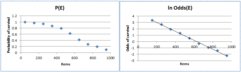
Figure 3 – Plot of probability and ln odds
Given that there is only one independent variable (namely x = # of rems), we can use the following model
![]()
Here we use coefficients a and b instead of b0 and b1 just to keep the notation simple.
We show two different methods for finding the values of the coefficients a and b. The first uses Excel’s Solver tool and the second uses Newton’s method. Before proceeding it might be worthwhile to click on Goal Seeking and Solver to review how to use Excel’s Solver tool and Newton’s Method to review how to apply Newton’s Method. We will use both methods to maximize the value of the log-likelihood statistic as defined in Definition 5.
Sample Size
The recommended minimum sample size for logistic regression is given by 10k/q where k = the number of independent variables and q = the smaller of the percentage of cases for y = 0 or y = 1, with a minimum of 100.
For Example 1, k = 1 and q = 302/760 = .397, and so 10k/q = 25.17. Thus a minimum sample of size 100 is recommended.
See Logistic Regression Sample Size for a more refined method of determining the minimum sample size required for logistic regression.
Examples Workbook
Click here to download the Excel workbook with the examples described on this webpage.
References
Howell, D. C. (2010) Statistical methods for psychology (7th ed.). Wadsworth, Cengage Learning.
https://labs.la.utexas.edu/gilden/files/2016/05/Statistics-Text.pdf
Christensen, R. (2013) Logistic regression: predicting counts.
http://stat.unm.edu/~fletcher/SUPER/chap21.pdf
Wikipedia (2012) Logistic regression
https://en.wikipedia.org/wiki/Logistic_regression
Agresti, A. (2013) Categorical data analysis, 3rd Ed. Wiley.
https://mybiostats.files.wordpress.com/2015/03/3rd-ed-alan_agresti_categorical_data_analysis.pdf
Hi Charles,
Can the analysis shown above be adapted for a multivariable approach? As in, can we just add in additional independent variables?
Best,
Scott
Hi Scott,
Yes, you can.
Charles
Where can I find the definitions of notation used in the logistic regression output?
Hi Bob,
What notation are you referring to since the output from logistic regression is not described on this webpage.
Information about the output can be found on the following webpage as well as other places.
https://www.real-statistics.com/logistic-regression/real-statistics-support-for-logistic-regression/
Charles
Sir,
A big thank for this great job. It is very useful to understand in deep logistic models.
I would like to know if raw data in example 1 are available? I would like to show that results with raw data are the same to results with aggregating data.
Thanks for this job.
Thierry
Yes, the data in example 1 is still available. In fact, you can download all the examples on the website by going to
Real Statistics Workbook Examples
Charles
Dear Charles
Sorry, I don’t understand understand how we get from the 2nd part of Definition 3, in which P(E)/(1-P(E)) is equal to the exponential of the regression equation to the 3rd part with P(E) on the left part of the equation. I am sure I would have got this once, but I seem to have forgotten the relevant maths. Any help would be gratefully received. Thank you, Mike.
Mike,
Let’s start with 1/[1+e^(-z)], which is equal to 1/[1+1/e^z]. Now multiply the numerator and denominator by e^z to get e^z/[e^z+1]. THis proves that e^z/[1+e^z] = 1/[1+e^(-z)], which is the form of the 3rd part of the equation.
Charles
Dr. Charles, good morning. Is it possible to apply the Aikike criterion (AIC), in multiple binary logistic regression models, to see which one has the best fit? and if possible how would you do it?
Thank you very much
Dr. Charles, buenos días. Es posible aplicar el criterio de Aikike (AIC), en modelos de regresión logistica binaria multiple, para observar cual tiene mejor ajuste? y si es posible como lo haría?
Muchas gracias
Hello Gerardo,
Yes, you can apply the AIC in binary logistic regression. The Real Statistics LogitRSquare function returns this value. See
Logistic Regression Functions
Charles
Thank you very much Dr. I had read but I had not stopped
Charles, Thanks again for your great work. In terms of Sample size calculation, when I calculate, actually I don’t know value of q since I have not started the experiment. How can I use formula 10*k/q? Thank you.
You need to make your best estimate based on past experience, previous studies, etc.
Charles
Ok, thank you!
Navy.
I am confused about the definition of L. You say it is the probability that “the sample data occurs as it does”.
But for a given category cat_i, if p_i is the probability to fall in cat_i; and n the number of trials for that category, the probability to observe n_i “success” is
\binom{n}{n_i}*p_i^n_i*(1-p_i)*(n-n_i) which would give rise to the product of the preceding formulas for i from 1 to k (k being the number of category).
But that’s not the way you define L. Am I right that here y_i is n_i/n ? Am I missing something? Of what L is the probability, precisely?
Olivier,
Regarding the definition of L, please see Maximum Log-Likelihood
Yes, y_i is n_i/n.
Charles
Charles, Thank you for great add-inn. Working with regression was never so easy.
Have a one, maybe silly from your experience perspective, question. How I can calculate 95%CI for regression coefficients ? I would like to plot the S curve and it’s lower & upper 95% bounds.
Thank you in advance for your help.
Marcin,
Glad to read that you find the Real Statistics addin useful.
You can read about how to calculate the standard error and confidence intervals at
https://real-statistics.com/logistic-regression/finding-logistic-regression-coefficients-using-excels-solver/
https://real-statistics.com/logistic-regression/significance-testing-logistic-regression-coefficients/
Charles
Charles,
Thanks for the amazing tool! I’ve tried your logit function on one of my data sets and found perfect agreement with other methods of calculating logit models. Very much appreciated!
I have a question on the applicability for another data set, in which the I have thousands of repeats on non-independent data. For example, we tested n participants on a test with a binary outcome with a number of independent variables (including repeats) in a fully repeated measures design. I’ve converted the binary outcome results into probabilities and done a multiple regression on the probabilities; however, I’m not satisfied with the resultant curve as for certain levels of the independent variables the regression model probability exceeds 1. Is it correct/justifiable to apply a logistic regression approach?
Andrew,
Sorry, but I don’t have a clear picture of your design.
Charles
Sorry that I wasn’t clear. I have data from a laboratory test with human subjects with several independent variables using a fully repeated measures design and a binary dependent variable. I’m unsure if it would be correct to use a logistic regression in this situation. Thanks
Andrew,
Sorry, but I don’t know what you mean by a fully repeated design.
Charles
Repeated measures in that all participants are tested under all combinations of independent variables, such that all manipulations are within subjects factors.
Andrew,
Based on what I understand about your situation, it seems like binary logistic regression could be a good choice.
In a previous comment, you said that the “levels of the independent variables the regression model probability exceeds 1”. This should not happen in logistic regression.
Charles
I was curious if you could provide some advice. Long forgotten are my ‘out-of-context’ statistics courses and having stumbled about your blog I hope make a comeback!
I’m looking to analyze the outcome of lots of simulations. At a high level I am comparing success vs failure of the simulation based on several different parameters. I want to get a report on the best parameter set to most likely have successful runs in the future.
In other words: y = f(x1,x2,x3,…,xn) where y is 0 or 1 and the x values are categorical (i.e., they only take on specific values though not the same number of options).
It seems logistic regression you described could be what I need but I could really use your 2cents on if I’m barking up the wrong tree. Thank you in advance!
Scott,
Although you haven’t provided me with enough information to say for sure, it does sound like logistic regression could be a suitable approach.
Charles
I do appreciate your feedback.
Thanks for the extraordinarily useful page. I’ve downloaded the examples-part 2 and am looking at the multinomial logit example 1. I apologize in advance for asking such a basic question, but if I look at the Odds calculated for cured for Dosage 20, Gender 0, we see 0 observed cured.
It isn’t clear to me how the Odds for cured could be anything other than zero.
As I say, it is a very basic question, thanks for an excellent site!
Richard, when you say “if I look at the Odds calculated for cured for Dosage 20, Gender 0, we see 0 observed cured”, are you referring to some worksheet on the website or to some other that you are working on? In general if the number of successes is 0, the the odds will be 0.
Charles
Hi Charles,
Say we are doing a binary logistic regression of y with respect to each of the separate variables x_1,x_2, x_3, i.e., we are logistically regressing x_1|y , x_2|y and x_3|y ; x_i is the independent variable in each case. Assume all pairs (b_i, b_j) have the same sign combination, i.e., b_i positive, b_j negative, etc.
Question: Is there a meaningful way of defining a new variable x from x_1,x_2, x_3 , say x=x_1+x_2+x_3 , so that we can regress x|y ? Specifically, here the x_i are measures of efficiency and y is a measure of control, so I want to measure the overall effect of control on efficiency.
Thanks in Advance.
Does the new variable have to be a linear combination of the independent variables?
Charles
I would prefer that it was, but it is not necessary. Could you please tell me for both cases, or please give me refs?
Thanks Again.
You can define a new variable p which is calculated as the formula for p on the following webpage
https://real-statistics.com/logistic-regression/basic-concepts-logistic-regression/
There is no linear version. The logit function shown on that webpage is linear.
Charles
Thanks a lot, Charles, very helpful.
I see, so please let me know if I am on the right track:
If we have Y regressed against, say, 1/3(X_1+X_2+X_3) , and we have our cutoff , say X_1>A, X_2>A, X_3>A (same for all ), then we want to model
P(E)/(1-P(E))
For E= Event that P(X_1=1 and X_2=1 and X_3=1 )? And here E is the event where each of X_1, X_2, X_3 are above their respective cutoff values, say x_1, x_2, x_3 respectively? Do we then need to know the joint distribution ? I think in this case it is safe to assume independence of the X_i.
Thanks Again.
Never mind, sorry, I just realized my mistake. Please feel free to delete my previous post.
When we deal with a time series data for x(i)s, among which collinearity is highly likely present, what model can I use to draw inference about the probability between x(i) and a binary dependent variable y(i) ?
Mich,
Sorry, but I don’t understand your question.
Charles
My appology. I used wrong term. The subject of my analysis is a pair of time series [ x(t), y(t) ], where y(i) is a binominal variable taking either value of 0 or 1. Does the presence of “serial correlation” and/or even “heteroskedascity” among x(t) breach any assumption of the model? If that is the case, do we have any resolution to carry out the logistic regression? Hope that this question makes sense. Sorry again.
Mich,
See page 13 and 14 of
http://people.stern.nyu.edu/jsimonof/classes/2301/pdf/logistic.pdf
Charles
Dear Charles
Thank you very much for the info. I really appreciate it.
Michio
Hi, Charles
Similar to the discussion on multiple linear regression, is there a discussion addressing outliers and influential observations in undertaking multiple logistic regression? Do you have a recommended suite of Real Statistics features that one should use?
Regards,
Rich
Rich,
I have not yet included this on the website or in the software, but I really should. I will look into this for a future release. In the meantime, here is an article that may be helpful:
http://scialert.net/fulltext/?doi=jas.2011.26.35&org=11
Charles
Hi, Charles
If you incorporate a discussion/tool for outlier detection in logistic regressions, perhaps you could include something on power as well?
Regards,
Rich
Rich,
I plan to add information about power and sample size for logistic regression. Just haven’t gotten to it yet.
Charles
Dear Charles,
I have followed your method using my data set, which has a sample size of ~500 and ~150 unique x-values, however only ~30 of the population died. This results in many infinity and negative infinity values for the ln Odds(E) graph. Is it still possible to create this graph and obtain the coefficients for the line of best fit?
My end goal is to create an ROC curve to find out how good the x-values are at predicting the outcome (lived/died).
Thanks a lot,
Ally
Ally,
I suggest that you create an example that adheres to the situation that you describe and try logistic regression to see what happens. My guess is that there is a good chance that it will still be possible to create the ROC curve that you are looking for.
Charles
Mr Charles,
The information you have provided here is truly helpful for someone like me who is studying statistics. Would you mind elaborating little bit how do we get the likelihood statistic as a binomial distribution?Thank you
Sorry, but I don’t understand your question. Are you looking for the likelihood statistic for the binomial distribution?
Charles
Apologies for not being clear with my question.I’m asking about the likelihood function which is used for evaluating the model.The formula which you have used to compare between the predicted probability and the actual outcome and which is converted to log likelihood statistic which is being maximized.The formula mentioned above definition 5 on this page.
Chirag,
I suggest that you look at the following webpage
https://real-statistics.com/general-properties-of-distributions/maximum-likelihood-function/
The idea is that the probability that the sample will occur as it does is a product of probabilities. This is because the sample elements are independent of each other; i.e. P(A and B) = P(A) x P(B) when A and B are independent events. Thus the likelihood function L is a product of probability function values (that are dependent on certain parameters). For logistic regression, the probability function is the pdf for the binary distribution.
Since the sample that was observed actually did occur, the approach we use is to find the values of the parameters that maximize L(i.e. that make the sample events most likely)
Charles
Dear Charles,
Greetings. As a novice, I must say I’ve found your website immensely helpful.
I have the following data which I need to build a regression model for. Kindly suggest how I might go about it…
Dependent Variable: Binary Categorical
Independent Variables: Many are categorical and many are interval
I need to see if it is possible to build a model and test it. Kindly advise.
Rahul,
Logistic regression is a possible choice. See the webpages on Logistic Regression.
Charles
I am so sorry for the last respond, it might be confusing because I forgot to put ‘0’
below is the data I am working on:
age leave stay total
18.6 0 2 2
18.8 2 0 2
18.9 1 0 1
19 1 0 1
19.1 0 1 1
19.2 2 1 3
19.3 0 1 1
19.4 0 1 1
19.5 1 0 1
19.6 0 2 2
19.8 4 2 6
19.9 1 1 2
20 2 2 4
20.1 3 4 7
20.2 1 3 4
20.3 4 1 5
20.4 5 9 14
20.5 3 4 7
20.6 3 7 10
20.7 4 6 10
20.8 4 8 12
20.9 5 16 21
21 7 8 15
21.1 5 10 15
21.2 5 13 18
21.3 7 16 23
21.4 6 17 23
21.5 14 13 27
21.6 12 13 25
21.7 12 17 29
21.8 17 9 26
21.9 7 23 30
22 20 32 52
22.1 19 32 51
22.2 21 49 70
22.3 23 55 78
22.4 25 36 61
22.5 27 46 73
22.6 22 54 76
22.7 32 31 63
22.8 32 50 82
22.9 50 39 89
23 39 65 104
23.1 40 81 121
23.2 42 89 131
23.3 44 80 124
23.4 71 66 137
23.5 50 84 134
23.6 64 94 158
23.7 57 95 152
23.8 59 108 167
23.9 77 88 165
24 61 105 166
24.1 66 118 184
24.2 70 131 201
24.3 73 114 187
24.4 66 108 174
24.5 64 137 201
24.6 62 159 221
24.7 66 135 201
24.8 86 130 216
24.9 96 126 222
25 82 152 234
25.1 75 135 210
25.2 88 143 231
25.3 72 149 221
25.4 92 156 248
25.5 89 171 260
25.6 95 173 268
25.7 80 172 252
25.8 103 150 253
25.9 94 183 277
26 92 156 248
26.1 95 185 280
26.2 97 196 293
26.3 86 179 265
26.4 95 208 303
26.5 72 187 259
26.6 94 169 263
26.7 89 195 284
26.8 84 167 251
26.9 86 157 243
27 83 181 264
27.1 90 177 267
27.2 75 187 262
27.3 76 191 267
27.4 75 206 281
27.5 72 197 269
27.6 66 207 273
27.7 84 150 234
27.8 77 174 251
27.9 59 152 211
28 67 166 233
28.1 64 164 228
28.2 64 174 238
28.3 65 165 230
28.4 82 200 282
28.5 80 195 275
28.6 78 179 257
28.7 83 155 238
28.8 89 148 237
28.9 74 150 224
29 68 153 221
29.1 69 125 194
29.2 71 180 251
29.3 67 156 223
29.4 55 187 242
29.5 75 164 239
29.6 63 151 214
29.7 58 164 222
29.8 58 143 201
29.9 64 146 210
30 62 111 173
30.1 55 159 214
30.2 66 160 226
30.3 54 147 201
30.4 49 149 198
30.5 58 141 199
30.6 50 163 213
30.7 50 179 229
30.8 51 143 194
30.9 52 129 181
31 56 136 192
31.1 46 138 184
31.2 40 134 174
31.3 65 147 212
31.4 49 145 194
31.5 58 125 183
31.6 34 184 218
31.7 51 136 187
31.8 43 125 168
31.9 47 116 163
32 43 129 172
32.1 43 115 158
32.2 52 142 194
32.3 41 114 155
32.4 42 132 174
32.5 61 137 198
32.6 45 157 202
32.7 50 127 177
32.8 43 117 160
32.9 50 114 164
33 49 120 169
33.1 32 129 161
33.2 35 117 152
33.3 51 134 185
33.4 41 131 172
33.5 49 131 180
33.6 40 154 194
33.7 39 101 140
33.8 36 135 171
33.9 45 108 153
34 42 92 134
34.1 41 115 156
34.2 48 114 162
34.3 40 117 157
34.4 38 132 170
34.5 40 114 154
34.6 25 134 159
34.7 27 110 137
34.8 52 96 148
34.9 35 106 141
35 38 89 127
35.1 23 103 126
35.2 38 90 128
35.3 34 101 135
35.4 34 106 140
35.5 38 108 146
35.6 45 112 157
35.7 25 103 128
35.8 37 91 128
35.9 22 84 106
36 31 93 124
36.1 37 81 118
36.2 18 90 108
36.3 39 91 130
36.4 26 96 122
36.5 30 98 128
36.6 33 102 135
36.7 28 71 99
36.8 27 74 101
36.9 28 64 92
37 33 74 107
37.1 19 78 97
37.2 25 81 106
37.3 31 72 103
37.4 27 88 115
37.5 31 89 120
37.6 25 83 108
37.7 25 69 94
37.8 16 88 104
37.9 28 64 92
38 19 43 62
38.1 23 54 77
38.2 25 73 98
38.3 21 71 92
38.4 19 76 95
38.5 21 64 85
38.6 17 70 87
38.7 27 68 95
38.8 21 63 84
38.9 18 66 84
39 16 54 70
39.1 22 59 81
39.2 20 72 92
39.3 14 45 59
39.4 17 69 86
39.5 19 72 91
39.6 16 65 81
39.7 12 64 76
39.8 16 51 67
39.9 12 42 54
40 15 59 74
40.1 19 41 60
40.2 10 59 69
40.3 10 57 67
40.4 18 60 78
40.5 17 77 94
40.6 17 51 68
40.7 13 60 73
40.8 13 51 64
40.9 19 52 71
41 10 66 76
41.1 22 61 83
41.2 8 63 71
41.3 19 37 56
41.4 16 51 67
41.5 13 56 69
41.6 15 75 90
41.7 9 54 63
41.8 19 56 75
41.9 14 50 64
42 16 51 67
42.1 15 52 67
42.2 13 59 72
42.3 12 56 68
42.4 22 62 84
42.5 16 67 83
42.6 13 84 97
42.7 9 82 91
42.8 15 67 82
42.9 19 63 82
43 19 70 89
43.1 21 74 95
43.2 17 83 100
43.3 12 80 92
43.4 17 73 90
43.5 13 73 86
43.6 10 75 85
43.7 15 72 87
43.8 13 69 82
43.9 9 59 68
44 12 69 81
44.1 12 79 91
44.2 14 71 85
44.3 12 87 99
44.4 9 72 81
44.5 11 82 93
44.6 14 83 97
44.7 14 68 82
44.8 14 55 69
44.9 12 77 89
45 11 72 83
45.1 7 63 70
45.2 13 61 74
45.3 9 65 74
45.4 12 64 76
45.5 12 75 87
45.6 15 71 86
45.7 7 68 75
45.8 9 47 56
45.9 13 57 70
46 10 41 51
46.1 12 46 58
46.2 12 43 55
46.3 16 44 60
46.4 9 55 64
46.5 6 45 51
46.6 12 41 53
46.7 10 47 57
46.8 3 36 39
46.9 8 44 52
47 8 34 42
47.1 9 35 44
47.2 13 41 54
47.3 4 51 55
47.4 11 41 52
47.5 7 31 38
47.6 3 55 58
47.7 3 43 46
47.8 8 37 45
47.9 8 30 38
48 8 36 44
48.1 7 33 40
48.2 6 31 37
48.3 5 27 32
48.4 6 35 41
48.5 6 38 44
48.6 9 38 47
48.7 4 27 31
48.8 5 37 42
48.9 9 29 38
49 6 25 31
49.1 10 24 34
49.2 8 35 43
49.3 6 31 37
49.4 5 33 38
49.5 5 27 32
49.6 6 31 37
49.7 4 30 34
49.8 6 30 36
49.9 7 27 34
50 2 20 22
50.1 13 24 37
50.2 4 32 36
50.3 3 28 31
50.4 3 22 25
50.5 1 32 33
50.6 1 24 25
50.7 5 24 29
50.8 4 20 24
50.9 4 22 26
51 1 14 15
51.1 2 23 25
51.2 3 21 24
51.3 4 16 20
51.4 3 16 19
51.5 3 22 25
51.6 5 20 25
51.7 3 14 17
51.8 2 20 22
51.9 4 11 15
52 3 18 21
52.1 4 12 16
52.2 2 11 13
52.3 2 13 15
52.4 2 14 16
52.5 7 11 18
52.6 4 13 17
52.7 1 25 26
52.8 5 6 11
52.9 2 11 13
53 5 11 16
53.1 1 7 8
53.2 2 11 13
53.3 1 14 15
53.4 2 28 30
53.5 6 9 15
53.6 3 10 13
53.7 2 13 15
53.8 5 8 13
53.9 1 8 9
54 0 8 8
54.1 1 12 13
54.2 0 3 3
54.3 0 12 12
54.4 0 7 7
54.5 2 6 8
54.6 1 7 8
54.7 0 12 12
54.8 0 9 9
54.9 0 5 5
55 8 3 11
55.1 49 1 50
55.6 1 1 2
55.7 0 1 1
55.8 1 1 2
55.9 1 0 1
56.1 1 0 1
56.4 0 1 1
56.5 0 2 2
56.6 0 1 1
56.7 1 0 1
56.9 0 1 1
57 2 0 2
57.1 1 0 1
57.3 0 1 1
57.8 0 1 1
58.5 0 1 1
58.7 1 0 1
60.6 1 0 1
61.2 1 0 1
70.7 0 1 1
Grand Total 10476 27764 38240
Thank you for your kindness, Sir.
Regard,
Please send me an Excel file with your data by email along with the results that you obtained that you say are different from mine. Please make sure that when you use the Real Statistics software that you don’t include the totals for each item in the input data range.
Charles
dear Mr. Charles,
I have sent an email to your address. Please kindly check.
regards,
Ikhlas
I wish to used this model to predict the attrition probability, but I wonder when seeing my P(E) and Odds(E) plot because it seems different from yours, do I need to check the data plot to decide whether my data could be modeling as binary logistic regression? if so, how to check it?
When you say that your P(E) and Odds(E) are different from mine, do you mean that you got a different answer for one of the examples on the website?
Charles
I am not using the example data, but I use mine, in the picture your P(E) and Odds(E) probability linearly decreasing by the x- axis getting bigger, but my data doesn’t, so my point is, is there any requirement when choosing the binary logistic regression as a model?
The assumptions are: the dependent variable has exactly two outcomes; observations are independent; no collinearity, outliers or high leverage/influencer values; the model fits (i.e. there is a linear relationship between the independent variables and the logit transformation of the dependent variable).
If you send me an Excel file with your data, I will try to figure out what is happening.
Charles
Dear Charles,
I’ve sent an email to you few days ago, please kindly review my data.
Best regard,
Ikhlas
Dear Ikhlas,
I haven’t forgotten your email, and will get to it shortly.
Charles
How do we get the P(E) values? Thank you.
The referenced webpage describes how to get the P(E) values. The webpage sometimes uses the notation p for P(E). The other webpages on the Logistic Regression topic gets into more detail. You can also download the spreadsheets with all the examples shown on the website to get even more information.
Charles
Thank you ????
I hope that my response was helpful. If not, please provide some more detail about what you are looking for.
Charles
I tried the logistic regression tool with a data-set of Rows-142829 and Columns- 47 and my system hangs each time. Please can you let me know what is the capability of the addin. Also recommend me some way i can apply logistic regression on the same.
Assuming that the data is in raw format (and not summary format), there are two possible approaches:
1. Try using the Logistic Regression data analysis tool, making sure that Raw data option is selected, but the Show summary in output option is not selected. To use the summary output option the number of rows must be less than 65,000.
2. If the above approach doesn’t work, use the LogitMatches function as described on the webpage https://real-statistics.com/logistic-regression/real-statistics-functions-logistic-regression/
With this amount of data, the analysis will be quite slow.
Charles
Dear Charles,
I was wondering how the sigmoid curve is plotted. It seems that the probabilty p given by p=1/(1+EXP(-B0-B1*x)) is plotted on the y-axis, what did you use on the x-axis? Seems to be from -3 to 3
Thanks in advance
Jip,
Yes, from -3 to 3.
Charles
Hi Charles, I’m trying to predict how suitable a prospective client would be for me; based on historical of my already existing clients. This will be based on 5 independent categorical variables.What do you suggest a suitable regression techniques would be?
You have several choices. First you need to decide whether your dependent variable is categorical or not.
If it is categorical then some version of logistic regression could be used. If there are two outcomes then the model is a binary logistic regression model (e.g. client is suitable or client is unsuitable). If there are multiple categories then you could use multinomial logistic regression or more likely ordinal logistic regression (e.g. client is a top prospect, client is a good prospect, client is a fair prospect or client is not a suitable prospect).
With only categorical variables you could also use log-linear models.
With a quantitative dependent variable (e.g. client is assigned a numeric rating from 0 to 100, with 100 representing clients that are most suitable), you could multiple regression employing dummy variables to handle the categorical independent variables.
All of these approaches are described on the Real Statistics website.
Charles
Dear Sir,
Thank You for your great explanations. Logic regression is used for item response theory also. Do you have any explanations about that?
Venura,
I don’t have any further information about this subject on the website. The site is evolving all the time and new information is constantly being added. What sort of explanations on this subject would be most helpful to you?
Charles
Sir,
we can use logistic regression in IRT to evaluate further students’ results,that’s what I asked.
Sorry Venura, I should have read your question more carefully. I now see that you are referencing item response theory. This is a topic that I need to add to the website.
Charles
In example 1, there’s a plot of the Odds(E). The plot shown looks to me like it is not the Odds(E), but rather the logit = ln Odds(E). Is this correct?
Alan,
Yes, you are correct. I have now changed the plot to ln Odds(E). Thanks for catching this.
Charles
Sir
I am at little confused about the value of yi in definition 5. In definition 5 you said yi is observed value. But I think if it is a binomial distribution y can only take the value of either 1 or 0, how could it be observed value of p?
Colin
Colin,
yi only takes a value of 0 or 1. pi is the predicted value, which can take any value between 0 and 1. Of course we will use the pi as a way of estimating the yi (even for unobserved yi). If pi > .5 (or some other preassigned value) then pi predicts a value for yi of 1 and pi < .5 predicts a value for yi of 0. Charles
Sir
I am sorry. I still don’t understand. In the “Finding Logistic Regression Coefficients using Excel’s Solver” you said yi “is the observed probability of survival in the ith of r intervals” and the value of yi in Figure 1 of “Finding Logistic Regression Coefficients using Excel’s Solver” does not take the value of either 0 or 1, which makes me confused.
Colin
Colin,
You are correct. It is a little confusing. I should have said that yi = the fraction of subjects in the ith interval that survived. I have now made this revision on the webpage.
Charles