Basic Concepts
Definition 1: For the binomial distribution the number of successes x is a random variable and the number of trials n and the probability of success p on any single trial are parameters (i.e. constants). Instead, we would now like to view the probability of success on any single trial as the random variable, and the number of trials n and the total number of successes in n trials as constants.
Let α = # of successes in n trials and β = # of failures in n trials (and so α + β = n). The probability density function (pdf) for x = the probability of success on any single trial is given by
![]()
This is a special case of the pdf of the beta distribution
![]()
where Γ is the gamma function.
Note that in the general case, α + β does not have to be a positive integer, although α and β do have to be positive numbers and x must be between 0 and 1.
Chart
A chart of the beta distribution for β = 8 and α = 2, 4 and 6 is displayed in Figure 1.
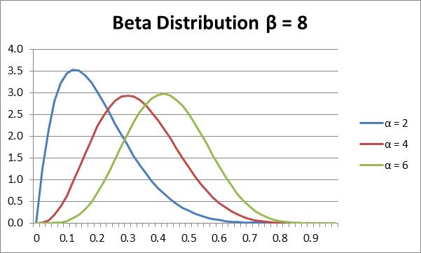
Figure 1 – Beta Distribution
Actually, the beta distribution can take a great variety of shapes, as shown in Figure 2.
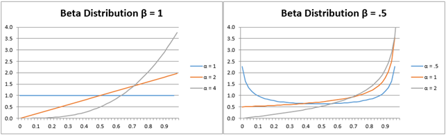
Figure 2 – Other shapes of beta distribution
Properties
Key statistical properties of the beta distribution are:

Figure 3 – Statistical properties of the beta distribution
The mode is (a) any value in (0,1) for α, β = 1, (b) 0 or 1 for α, β < 1, (c) 0 if α ≤ 1 and β > 1 and (d) 1 if β ≤ 1 and α > 1.
Excel Worksheet Functions
Excel Functions: Excel provides the following functions:
BETA.DIST(x, α, β, cum) = the pdf of the beta function f(x) when cum = FALSE and the corresponding cumulative distribution function F(x) when cum = TRUE.
BETA.INV(p, α, β) = x such that BETA.DIST(x, α, β, TRUE) = p. Thus BETA.INV is the inverse of the cdf of the beta distribution.
These functions are not available in versions of Excel prior to Excel 2010. Instead, these versions of Excel use BETADIST(x,α,β), which is equivalent to BETA.DIST(x,α,β,TRUE), and BETAINV, which is equivalent to BETA.INV.
Observations
Note the following equality when s and n are positive integers with n > s:
BETA.DIST(p, s, n-s, TRUE) = 1 – BINOM.DIST(s-1, n-1, p, TRUE)
The cdf of the beta distribution is also called the regularized incomplete beta function, denoted Ix(α,β). Thus, Ix(α,β) = BETA.DIST(x, α, β, TRUE).
Example
Example 1: A lottery organization claims that at least one out of every ten people wins. Of the last 500 lottery tickets sold 37 were winners. Based on this sample, what is the probability that the lottery organization’s claim is true: namely that players have at least a 10% probability of buying a winning ticket? What is the 95% confidence interval?
To answer the first question we use the cumulative beta distribution function as follows:
BETA.DIST(.1, 37, 463, TRUE) = 98.1%
This represents that organization’s claim is false (i.e. less than 10% probability of success). The probability that the organization’s claim is true is only 100% – 98.1% = 1.9%.
The lower bound of the 95% confidence interval is
BETA.INV(.025, 37, 463) = 5.3%
The upper bound of the 95% confidence interval is
BETA.INV(.975, 37, 463) = 9.8%
Since 10% is not in the 95% confidence (5.3%, 9.8%), we conclude (with 95% confidence) that the lottery’s claim is not accurate.
Real Statistics Worksheet Functions
Real Statistics Function: The Real Statistics Resource Pack provides the following function:
BETA(α, β) = the beta function = Γ(α)Γ(β)/Γ(α+β)
Thus, the pdf of the beta distribution is
![]()
Four-parameter Distribution
Observation: The two-parameter version of the beta distribution, as described above, is only defined for values of x between 0 and 1. There is also a four-parameter version of the distribution for which x is defined for all x between a and b where a < b.
The cdf for the four-parameter beta distribution at x is F(z) where F is the cdf for the two-parameter distribution and z = (x–a)/(b–a). The pdf at x is
![]()
Excel Functions: Excel provides the following functions to support the four-parameter version of the beta distribution.
BETA.DIST(x, α, β, cum, a, b) = the pdf of the beta function f(x) when cum = FALSE and the corresponding cumulative distribution function F(x) when cum = TRUE.
BETA.INV(p, α, β, a, b) = x such that BETA.DIST(x, α, β, TRUE, a, b) = p; i.e. the inverse of the cdf of the beta distribution.
These functions are not available in versions of Excel before Excel 2010. Instead, these versions of Excel use BETADIST(x, α, β, a, b), which is equivalent to BETA.DIST(x, α, β, TRUE, a, b), and BETAINV, which is equivalent to BETA.INV.
Beta Prime Distribution
Click here for information about the beta prime distribution.
Examples Workbook
Click here to download the Excel workbook with the examples described on this webpage.
References
Taboga, M. (2017) Beta distribution. Lectures on probability theory and mathematical statistics, Third edition. Kindle Direct Publishing
https://www.statlect.com/probability-distributions/beta-distribution
Wikipedia (2020) Beta distribution
https://en.wikipedia.org/wiki/Beta_distribution
Is the Real Statistics BETA function compatible with the first formula shown on this page (the formula right under “A/B testing: binary outcomes”)?:
https://www.evanmiller.org/bayesian-ab-testing.html
Thank you.
Hello Steven,
The Real Statistics BETA function is equivalent to the B function on that page.
Charles
Thanks for sharing. Could we not have tested the lottery organisation’s claim by just building a binomial model with p = 0.1, calculating P(X ≤ 37), and rejecting the null hypothesis at a chosen significance level, say 5%?
LM,
First of all, the scenario is not for p = .1, but for any value of p >= .1.
Charles
Hi Charles,
I have the following set of data (18) and trying to find the best fit assuming Beta distribution:
2 2.4 2.6 2.9 3.1 3.9 3.9 3.9 4.1 4.1 4.2 4.6 4.6 4.7 4.9 4.9 5 5
Please can you assist. Thanks a lot.
Ronald
Ronald,
See https://www.real-statistics.com/distribution-fitting/
Two methods are described for the beta distribution. Usually, the MLE approach is better.
Charles
Hi charles im not too much good in statistics, however i am very obsessed with non normal distribution. Since i am developing an excel file which i want to be very dynamic and sensitive with the skewed plot. I have some questions;
1. Could be the beta distribution able to show or represent a negative skewed graph? (i learnt gamma distribution only show positive skewed)
2. If i have a set of data (assumed it is negative skewed) ranging from cell A1:A1000, how can i compute for a”alpha” and B”beta” to be filled in the “=beta.dist(x,a,B,cum)”? (i learnt that “a = mean^2 / variance” and “b = variance / mean” which fits a gives me a good graph in the funtion gamma.dist in excel, however using it in beta.dist gives me an error result)
In connection with question number 2, i forgot to tell that the range cell A1:A1001 is a set of ungrouped raw data (assumed to be skewed).
Cell B1 “=average(a1:a1001)
Cell B2 “=stdev.s(a1:a1001)
Then, on cell C1:C21 i grouped them into 20 classes
Cell C1 “=B1-(10*B2)
Cell C2 “=C1+$B$1
Drag down C2 upto C21
Now on D1:D21 i want to get their “=beta.dist(C1,a,B,cum)
a=?
B=?
If the approach suggested in my previous response is not appropriate, then perhaps you can get the answer using Solver.
Charles
1. Using a for alpha and b for beta, the skewness of the beta distribution is 2*(b-a)*Sqrt(a+b+1)/(a+b+2)*Sqrt(ab)). Thus, you can choose appropriate values of a and b to obtain the type of skewness that you desire (if it exists).
2. The Real Statistics website describes two methods for fitting a beta distribution to some data. See the following webpages:
https://real-statistics.com/distribution-fitting/method-of-moments/method-of-moments-beta-distribution/
https://real-statistics.com/distribution-fitting/distribution-fitting-via-maximum-likelihood/fitting-beta-distribution-parameters-mle/
If an error is returned it might mean that the data can’t be fit by a beta distribution
Charles
Thank you so much charles
Another question, could you site any distribution that may fit with the negatives skewed histogram
See https://stats.stackexchange.com/questions/89179/real-life-examples-of-distributions-with-negative-skewness
Charles
Hi, this is probably trivial to people who know statistics well, but can you please explain/give reference to the following statement in the text:
The probability density function (pdf) for x = the probability of success on any single trial is given by
https://i1.wp.com/www.real-statistics.com/wp-content/uploads/2012/11/beta-distribution-pdf.png
See the following webpage for an explanation:
https://www.statlect.com/probability-distributions/beta-distribution
The following webpage may also be helpful:
https://stats.stackexchange.com/questions/4659/relationship-between-binomial-and-beta-distributions
Charles
Hi,
when calculating the lower and upper bounds -> if the sample size is small, one should use the following formulas:
alpha – confidence interval
k – number of successes
n – number of trials
lower: BETAINV((1-alpha)/2, k, n-k+1)
upper: BETAINV((1+alpha)/2, k+1, n-k)
however, i’m not sure, if any changes should be applied to the BETADIST function.
Matijia,
What is the reference for the statement “if the sample size is small, one should use the following formulas…”?
Charles
i want to find out activity weightage and Quantity , through calendardate , here I will create report like below
start date finish date activity calender
weightage
01/09/2021
are given , 02/01/20 20/04/20 94.4
to create formule in Beta distribution
Sorry, but I don’t understand your question.
Charles
Matijia,
Thank you for providing these equations. Using them, I was able to match the behavior of the Matlab binofit() function.
Andrew
Thank you Charles ..
However May i know what is the application of this charts
regards
Raj
Raj,
To provide a sense of what the distribution looks like and what is the effect of changing a parameter value.
Charles
How did we get the graphs in the Beta distribution. can you please explain
Raj,
Enter 2 in cell B1, 4 in cell C1 and 6 in cell D1.
Next enter 0 in cell A2 and the formula =A2+.02 in cell A3. Highlight the range A3:A51 and press Ctrl-D.
Now insert the formula =BETA.DIST(B2,B$1,8,FALSE) in cell B2. Highlight range B2:D51 and press Crtl-R and then Ctrl-D.
This completes all the data. You now create the chart by highlighting range and selecting Insert > Charts > Line Chart.
You can then add titles and make other modifications as described on the webpage
Excel Charting
Charles
I used Exact Excel method to calculate the two sided CI (95% Confidence Level) as below. It is equivalent to “Clopper Pearson” method.
The upper bound is BETAINV(0.975, 38, 463) =10.1%. The lower bound is BETAINV(.025, 37, 464) = 5.3%.
In this case, 10% is in the CI (5.3%, 10.1%), we can conclude that the lottery’s claim is accurate.
In sum, the exact method uses α=38 instead of 37 used in the upper bound. In contrast, using the exact method draws a different conclusion although the two set of confidence limits are very close. There is statistical significance but no practical significance.
Charles,
First, thanks for devoting time to set up that website, it is a goldmine!
In your lottery example (nber 1) above, could we also use the Binomial Distribution to compute the probability to observe 37 or less winning tickets if the underlying probability is 10%?
So, =BINOM.DIST(37,500,0.1,1)?
Many thanks in advance Charles,
Fred
Fred, BINOM.DIST(37,500,.1,1) = .02743, which means that the probability of getting 37 or fewer winning tickets out of 500 is 2.743% when the probability of getting a winning ticket (on any one ticket) is 10%. This doesn’t answer question 1.
Charles
Thank you! I was looking at it from the point of view of hypothesis testing, We would reject H0: p=0.1 because p-value=0.02743 <0.05?
You should really self-publish an e-book version of the website on Amazon.
Thanks again!
Fred
Hello there,
For some reason, the equations on all webpages are not displayed. May be some background maintenance is underway; just wanted to bring to your attention.
Thanks!
Thanks for bringing this to my attention.
I don’t know why the equations were not displayed. I see that they are displayed now (at least on my computer).
Charles
Nice job Charles. That is a sweet explanation. I saved the webpage. Thanks! If this is a book, I need a copy!
Karl,
There will be a series of books shortly.
Charles
I am a little confused how Bayesian updating is carried out for the following set-up:
I have developed a logistic regression model which provides % probability of a 1 or 0. The 1 or 0 is then compared to what actually happened and a Beta Distribution is updated for each new success or failure which provides % probability of successes (1s).
I now which to use my Logistic Regression model which new data to provide a new % estimate of a 1. This in turn now needs to be updated with the previously calculated probability from the Beta distribution calculated on the previous time step.
How should I use Bayes to update the current Logistic regression probity with the actual % wins/losses? I am confused as which one is the prior and psoterior?
Thanks for the help.
Adam
Sorry Adam, but I really don’t understand the scenario that you are describing.
Charles
I believe Adam was referring to how the Beta distribution is often used iteratively in Bayesian stats. It can be explained as the probability of probabilities. E.g. what are the chances of having a final sample mean of 0.3 if the current sample mean is 0.27 with 2 out of 9 iterations remaining.
The usual example is baseball, see http://varianceexplained.org/statistics/beta_distribution_and_baseball/, but your lottery example works.
In summary, if we approach the goal at a faster rate than expected then we are more likely to meet or exceed that goal. And if we fall behind the less likely we are to are to meet it.
Anthony,
Thanks for your explanation.
Charles
how the alpha and beta values are to be taken for a problem.
please explain me.
thank you
For the problem described on the referenced webpage, α = # of successes in n trials and β = # of failures in n trials (and so α + β = n).
Charles
Hi,
When there are 0 successes or n successes (out of n trials), the formula returns #NUM!
Do you have a work around for this? As in the situation where we had 100 trials and 0 successes we could safely assume that the probability of success was close to 0 – but this formula would not give an interval.
oops – I forgot to mention that I am talking about estimating confidence intervals using the beta.inv(p,alpha,beta) formula. Thank you
John,
Note that BETA.DIST(p, s, n-s, True) = 1 – BINOM.DIST(s-1, n-1, p, True).
Thus, BETA.DIST(p, 0, 100, True) = 1 – BINOM.DIST(-1, 99, p, True).
This means that the problem you are addressing is equivalent to asking (the binomial distribution question) what is the probability of getting -1 successes in 99 trials (for any value of p = probability of success on any single trial)? This is clearly 0 with a confidence interval consisting only of the point zero. Thus the confidence interval you are looking for is [1,1], i.e. the point 1.
Charles
“Thus the probability that the organization’s claim is true is 100% – 98.1% = 1.9%”
This sure sounds like the inverse probability error.
Pr(.074 | π = .1) = .019
does not mean
Pr(π = .1 | .074) = .019
Would it not be better to say that obtaining p < 37/500 = .074 would occur only 1.9% of the time if the organization’s claim (H0: π = .1) were true?
Rick
Rick,
While you are right to be cautious, I believe the logic used is correct.
Pr(π < .1 | # of successes in 500 trials = 37 and # of failures in 500 trials) = BETADIST(.1, 37, 463) = 98.1% Thus Pr(π >= .1 | # of successes in 500 trials = 37 and # of failures in 500 trials) = 1 – 98.1% = 1.9%
Charles
I noticed that in this example, assuming 50 wins and 450 losses, so exactly 10%, yields:
BETADIST(.1, 50, 450) = 51.6%
and increasing the sample size to e.g. 5000 out of 45000 or higher, only leads to values closer and closer to 50%.
With the stated logic there would always be at least a 50% chance the claimed chance of 10% wins is a fraud.
Could it be that the correct calculation for 50 out 500 is the following:
2*(51.6% – 50%) = 3.2% chance of a lie
And with your example 37 out of 463:
2*(98.1% – 50%) = 96.2% chance of a lie
This way the whole range from 0% to 100% truth or lie is possible and entering the promised 10% wins approaches 0% chance of a lie with increasing sample size.
Not sure about this, though.
Thank you for the helpful article!
Matthias,
I don’t know what you mean by “exactly 10%” in your first sentence. I also don’t know what you mean by “a lie”. Sorry, but I also don’t understand the calculations. Let me review a few things.
BETADIST(.1, 50, 450) is the cumulative probability distribution function and is equal to 51.59%. This means that given that we have observed 50 winners in 500 lottery tickets, the probability that any single ticket has up to a 10% chance of winning is 51.59%. Note that I have said “up to a 10% chance of winning” and not “exactly a 10% chance of winning”. All this is difficult to interpret since we have two levels of probability.
The chance that any single ticket has more than a 10% of winning is therefore 48.41%. Thus, it is more likely that any single ticket is a winner less than 10% of the time than more than 10% of the time, but the difference is close (and so my be due to chance).
Note that if you increase the sample size to 5000, but keep the 50 fixed, then BETADIST(.1,50,4950) = 1, which is what you would expect since it seems pretty unlikely that 10% of the tickets are winners given that only 50 out of 5,000 were winners. In fact, note that BETADIST(.01,50,4950) = 51.86%.
Charles
Good and simple explanation of beta distribution compared to 99% sites I looked.Could you tell why we place (n-1)! in the numerator when the number of trials will always be an whole number.It might be certain to have (\alpha-1)! and (\beta-1)! in the denominator since and might be real numbers.Also why isn’t the power of x and (x-1) in the numerator \alpha and \beta instead of (\alpha-1) and (\beta-1) given in the expression?
Justin,
The only time I need to use the beta distribution on the website is when the alpha and beta values are integers, although the beta distribution is used for many other purposes, including cases where the alpha and beta parameters are not integers. The distribution uses the gamma function. You see a number of instances of some integer minus 1. The reason for this is that Gamma(n) = (n-1)! when n is a positive integer.
Charles
I like your derivation (whenever I have seen this done previously, it has been through repeated application of integration by parts on the cdf, and is much more complicated), but I have a similar problem to Justin. To go from the pdf
f(x) = n!/k!/(n-k)!*x^k*(1-x)^(n-k)
I would have to set a-1=k and b-1=n-k, which gives
f(x) = n!/(a-1)!/(b-1)!*x^(a-1)*(1-x)^(b-1)
and is therefore not the same as the first of your equations above (by a factor of n). Do you see where I’m going wrong?
Richard,
First note that Gamma(m) = (m-1)! for any positive integer m. Thus for any positive integers alpha and beta, (alpha-1)! = Gamma(alpha) and (beta-1)! = Gamma(beta). Now let n = alpha + beta. Then (n-1)! = Gamma(n) = Gamma(alpha+beta).
Putting the pieces together yields (n-1)!/((alpha-1)!*(beta-1)!) = Gamma(alpha+beta)/(Gamma(alpha)*Gamma(beta)).
This is not the same thing as deriving the cdf from the pdf.
Charles
I used Beta Distribution Equation in Excel but result not same of Beta.Dist…Why
Sadam,
BETADIST calculates the cumulative distribution function (cdf) F(x), while the formula is for the probability density function (pdf) f(x).
BETA.DIST(x,alpha,beta,FALSE) will calculate the pdf.
Charles