Lorenz Curve

Basic Concepts

The Gini index is related to the Lorenz curve y = L(x). The x and y values for this curve are in the range of 0 to 1. If we are measuring income, for example, then if z_max is the maximum income that anyone in the population earns (and 0 is the theoretical minimum earnings), then for any income amount z (between 0 and z_max), if x is the percentage of the population that has income less than or equal to z, then y = L(x) = z/z_max.

This curve always lies below the curve y = x, which represents the equality curve, i.e. where every member of the population has the same y value.

Example

Example 1: Draw the Lorenz curve for the data in range A4:A23 in Figure 1.

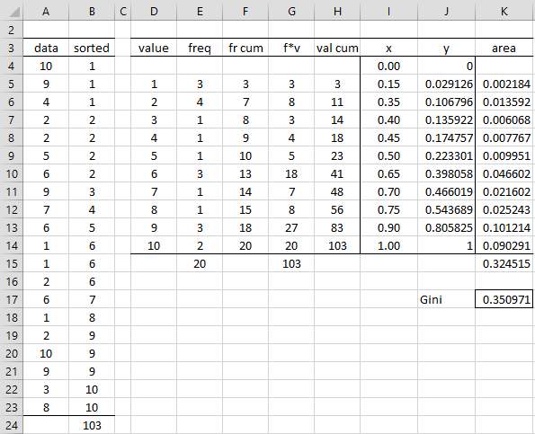
Figure 1 – Data for Lorenz Curve and Gini Index

The first thing we need to do is sort the data in ascending order. This is done in column B, for example by using the Real Statistics array formula =QSORT(A4:A23) in range B4:B23. We now create a frequency table by placing the unique data values in column D. If there are no replications in column B, then column D is the same as column B.

Calculating the x values

For this example, it is clear from column B that the unique data values are the values 1 through 10. If it is not so obvious, we can place the Real Statistics array formula =NODUPES(B4:B23) in range D5:D14. Actually, we can use the Real Statistics array formula =SortUnique(A4:A23 instead, in which case, we don’t need column B at all.

The values in column E represent the frequency values corresponding to the values in column D. E.g. the data value 1 occurs three times and so the frequency value in cell E5 is 3. This can be obtained by using the Excel array formula =COUNTIF($A$4:$A$23,D5). The other frequency values can be obtained by highlighting the range E5:E14 and pressing the key sequence Ctrl-D. The sum of all the frequency values is 20 (cell E15), as calculated by =COUNT(A4:A23) or =SUM(E5:E14).

Column F contains the cumulative frequencies. Here, we place the formula =E5+F4 in cell F5, highlight range F5:F14, and press Ctrl-D. If we divide each of these values by 20, we get the x values for the Lorenz curve, as shown in column I. Here, we place the formula =F4/E$15 in cell I4, highlight the range I4:I14, and press Ctrl-D.

Calculating the y values

We now show how to calculate the corresponding y values for the Lorenz curve. First, we place the formula =D5*E5 in cell G5 and =G5+H4 in cell H5. We can now fill in the other values in columns G and H as we have done previously, with cell G15 containing the sum of all the original data values, as calculated by =SUM(A4:A23) or =SUM(G5:G14).

The y values for the Lorenz curve, shown in column J, are the cumulative data values from column H divided by the sum of all the data values from cell G15. This is done by placing the formula =H4/G$15 in cell J4, highlighting the range J4:J14, and pressing Ctrl-D.

Graph of Lorenz curve

We now use Excel’s charting capabilities to obtain the graph of the Lorenz curve shown in Figure 2. We also include the y = x curve representing the equality curve.

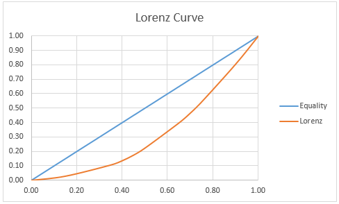
Figure 2 – Lorenz Curve

Highlight range I4:J14 and select Insert > Charts|Scatter and pick the Scatter with Smooth Lines option. Next, select Design > Data|Select Data to produce the dialog box shown in Figure 3.

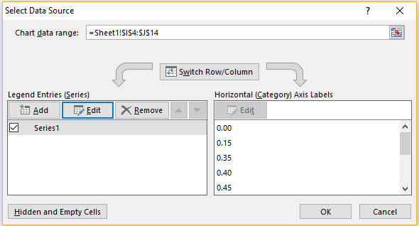
Figure 3 – Select Data Source dialog box

First, click the Add button on the left side of the dialog box. Fill in the dialog box that appears as shown in Figure 4 and click on the OK button.

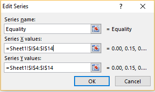
Figure 4 – Add Equality series

Note that you are entering the same values for the Series X values as the Series Y values (since the x and y values are the same on the line y = x). When the dialog box in Figure 3 reappears, click on Series1 on the left side of the dialog box and click on the Edit button to change the Series1 label to Lorenz.

After adding the chart title, making sure the Legend is displayed and ensuring that the x-axis and y-axis run from 0 to 1 (as explained in Excel Charts), you arrive at the chart shown in Figure 2.

Gini index as the area under Lorenz curve

The Gini index is equal to twice the area between the Equality and Lorenz curves. Note that the area under the Equality curve is 0.5 and the area under the Lorenz curve can be approximated by adding the areas of trapezoids as described in ROC Data Analysis Tool. The area of the 10 trapezoids used for Example 1 is shown in column K of Figure 1. E.g. the area of the first trapezoid (cell K5) is calculated by the formula =(I5-I4)*(J5+J4)/2. To calculate the area of the other trapezoids, highlight the range K5:K14 and press Ctrl-D.

The area under the Lorenz curve is approximately .3415, the sum of these areas (cell K15), as calculated by the formula =SUM(K5:K14). The area between the curves is therefore .5 – .3245 = .175. The Gini index is, therefore, twice this value, namely .351, as shown in cell K17. Note that since the area under the Equality curve is .5, the Gini index measures the percentage less than perfect equality represented by the data, which for Example 1 is 35.1%.

Gini index calculation

We can also calculate the Gini index using the formula

as described in Gini Coefficient. This calculation is illustrated in Figure 5.

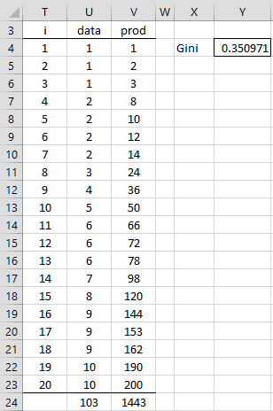
Figure 5 – Alternative Gini calculation

Here, column T contains the indices from 1 to 20, and column U contains the data in ascending order (i.e. a copy of column B from Figure 1). Column V contains the product of the values in columns T and U(e.g. cell V4 contains the formula =T4*U4) and cell V24 contains the sum of the elements in column V. Finally, the Gini index of .351 (cell Y4) is calculated by the formula

=2*V24/(T23*U24)-(T23+1)/T23

Note that you can calculate the Gini index using the following directly from the unsorted raw data, range A4:A23 from Figure 1:

=(2*SUMPRODUCT(SEQ(COUNT(A4:A23)),QSORT(A4:A23,,-1))/ SUM(A4:A23)-(COUNT(A4:A23)+1))/COUNT(A4:A23)

Here, QSORT and SEQ are Real Statistics functions. In Excel 2019 or 365, SEQ can be replaced by the standard Excel function SEQUENCE.

Worksheet Function

Real Statistics Function: The following function is provided in the Real Statistics Pack:

GINI(R1): the Gini coefficient for the data in R1

The data in R1 does not need to be in sorted order. For Example 1, =GINI(A4:A23) produces the value in cell Y4 of Figure 5.

Examples Workbook

Click here to download the Excel workbook with the examples described on this webpage.

References

Mirzaei, S., Borzadaran G. R. M., Aminib, M., Jabbarib, H. (2017) A comparative study of the Gini coefficient estimators based on the regression approach. Communications for Statistical Applications and Methods. Vol. 24, No. 4, 339–351.
http://www.csam.or.kr/journal/download_pdf.php?doi=10.5351/CSAM.2017.24.4.339

Buchan, I. E. (2016) Gini coefficient of inequality. Stats Direct Limited
https://www.statsdirect.com/help/nonparametric_methods/gini_coefficient.htm

Wikipedia (2019) Lorenz curve
https://en.wikipedia.org/wiki/Lorenz_curve